Planning repeated surveys and panels

A repeated survey can target a level at one occasion, a change between occasions, or an average across occasions. Sharing units across occasions has different consequences for those estimands. This article connects those precision questions to panel recruitment and fieldwork schedules.

See Getting started for single-occasion sizing and Power for detecting a change.

Terms used here

Term	Meaning
Occasion	One calendar round of the survey.
Wave	A unit’s interview number within its participation period.
Cohort	Units entering the design together.
Retention	Conditional probability of remaining from one wave to the next.
Issued overlap	Share of selected units common to two occasions.
Respondent overlap	Share of the first occasion’s respondents measured again.

Keep issued and respondent overlap separate whenever response is incomplete.

Precision for change

n_change() and prec_change() plan a change in a mean or proportion. Start with independent samples at the two occasions:

n_change(p = c(0.30, 0.36), moe = 0.02)
#> Sample size for change (proportion scale)
#> n = 4230 per occasion (p = 0.3 to 0.36, moe = 0.02, deff = 1)
#> No between-occasion covariance (overlap x overlap_cor = 0)

Measuring some of the same responding units at both occasions reduces the variance of a difference when their measurements are positively correlated:

change_plan <- n_change(
  p = c(0.30, 0.36),
  moe = 0.02,
  overlap = 0.75,
  overlap_cor = 0.50
)
change_plan
#> Sample size for change (proportion scale)
#> n = 2646 per occasion (p = 0.3 to 0.36, moe = 0.02, deff = 1)
#> overlap = 0.75, overlap_cor = 0.5 (62.5% of the independent variance)
prec_change(change_plan)
#> Sampling precision for change (proportion scale)
#> n = 2646 per occasion (p = 0.3 to 0.36, deff = 1)
#> overlap = 0.75, overlap_cor = 0.5 (62.5% of the independent variance)
#> se = 0.0102, moe = 0.02, cv = 0.1701, rmoe = 0.3333

overlap is a design property. overlap_cor is specific to the outcome and should come from an earlier round or other defensible evidence. A full panel with zero outcome correlation provides no variance reduction for change.

Precision for an average across occasions

An annual average of quarterly estimates is a different estimand. Positive covariance is subtracted in a difference but added in an average:

prec_pooled(var = 100, n = 500, occasions = 4)
#> Sampling precision for pooled estimate (mean scale)
#> n = 500 per occasion, 4 occasions (var = 100, deff = 1)
#> No between-occasion covariance (overlap x overlap_cor = 0)
#> se = 0.2236, moe = 0.4383
prec_pooled(
  var = 100,
  n = 500,
  occasions = 4,
  overlap = 0.75,
  cor_decay = 0.80
)
#> Sampling precision for pooled estimate (mean scale)
#> n = 500 per occasion, 4 occasions (var = 100, deff = 1)
#> overlap = 0.75, overlap_cor = 0.8 at lag 1, shared out to lag 3
#> se = 0.3586, moe = 0.7029

In the second calculation, adjacent occasions share 75% of units and outcome correlation decays as 0.8^m at lag m. Under the ordinary case where overlap exceeds the sampling fraction, sharing units sharpens change estimates but reduces the information gained by averaging occasions. A single-occasion level depends on that occasion’s sample size and is unchanged.

The length of participation is the design lever that sets the overlap. Take the overlaps from rotations that keep a unit in sample for 2, 4, 6, or 8 consecutive occasions, and compare the standard errors at the same occasion sample over an eight-occasion horizon:

horizon <- 8
arms <- function(life) {
  rot <- design_rotation(as.character(life))
  ov <- design_overlap(rot, max_lag = horizon - 1)
  data.frame(
    span = attr(rot, "life"),
    interviews = attr(rot, "n_occasion"),
    overlap_1 = round(as.numeric(ov)[1], 3),
    se_level = round(prec_mean(var = 100, n = 1000, N = 1e5)$se, 4),
    se_change = round(prec_change(
      var = 100, n = 1000, N = 1e5,
      overlap = ov[1], overlap_cor = 0.80
    )$se, 4),
    se_pooled = round(prec_pooled(
      var = 100, n = 1000, N = 1e5,
      occasions = horizon, overlap = ov, cor_decay = 0.80
    )$se, 4)
  )
}
do.call(rbind, lapply(c(2, 4, 6, 8), arms))
#>   span interviews overlap_1 se_level se_change se_pooled
#> 1    2          2     0.500   0.3146    0.3458    0.1447
#> 2    4          4     0.750   0.3146    0.2821    0.1820
#> 3    6          6     0.833   0.3146    0.2574    0.2018
#> 4    8          8     0.875   0.3146    0.2441    0.2131

Reading down the columns, longer participation sharpens the change estimate and blunts the pooled average. The single-occasion level does not move, because it depends only on that occasion’s sample size. It is a reference line rather than a third position on the trade-off, which runs between change and the average. span counts the occasions from a unit’s first interview to its last, and interviews counts how often it is asked. They coincide here because each rotation is uninterrupted.

The table assumes full response. That is the only case in which prec_pooled() accepts a design_overlap() result directly. Below full response it refuses the issued overlap and asks for the respondent overlap you expect.

Neither estimand dominates, so a design serving both change and pooled estimates takes the larger of the n_change() and n_pooled() requirements:

change_required <- n_change(
  var = 100,
  moe = 1.5,
  overlap = 0.75,
  overlap_cor = 0.80
)
pooled_required <- n_pooled(
  var = 100,
  moe = 1.5,
  occasions = 4,
  overlap = 0.75,
  cor_decay = 0.80
)

requirements <- c(
  change = as.double(change_required),
  pooled = as.double(pooled_required)
)
requirements
#>   change   pooled 
#> 136.5852 109.7804
max(requirements)
#> [1] 136.5852

?prec_pooled documents the finite-population boundary where overlap falls below the sampling fraction. The function checks the complete covariance matrix rather than returning a variance from an invalid combination.

prec_pooled(
  var = 100,
  n = 67000,
  occasions = 8,
  N = 1e5,
  overlap = design_overlap(design_rotation("4"), max_lag = 7),
  cor_decay = 0.80
)
#> Error:
#> ! the assembled between-occasion covariance is not a valid covariance (minimum eigenvalue -1.55e-05 against a diagonal of 0.000493); at a sampling fraction of 0.67 the covariance at lag 2 is negative, which happens once a lag's overlap falls below n/N. Over 8 occasions a rotation interviewing each cohort 4 times at this size draws 1.34 times the population, so the schedule could not be fielded either. Reduce the sampling fraction, shorten the horizon, or supply an overlap and correlation that hold together across lags

This diagnostic identifies the lag at which the covariance changes sign and whether the rotation would also exhaust the population over the horizon.

Derive overlap from a rotation

design_rotation() records the occasions a cohort is in and out of sample. The string "4-8-4" means four occasions in sample, eight out, and four more in sample before leaving permanently:

cps_rotation <- design_rotation("4-8-4")
cps_overlap <- design_overlap(cps_rotation)
cps_overlap[c(1, 12)]
#> [1] 0.75 0.50

The results are the 75% month-to-month and 50% year-to-year issued overlaps of the Current Population Survey design (U.S. Census Bureau and U.S. Bureau of Labor Statistics 2019). The specification describes one cohort’s finite participation pattern. It is not an endlessly repeating cycle.

A rotation records two measures of respondent burden. The life attribute is the span from a unit’s first interview to its last, and n_occasion counts the interviews. They separate when the pattern has a rest period:

c(
  span = attr(cps_rotation, "life"),
  interviews = attr(cps_rotation, "n_occasion")
)
#>       span interviews 
#>         16          8

The "4-8-4" pattern spans sixteen occasions and asks each unit eight times.

Use the overlap for the lag being estimated:

c(
  consecutive = n_change(
    p = c(0.30, 0.36), moe = 0.02,
    overlap = cps_overlap[1], overlap_cor = 0.50
  )$n,
  annual = n_change(
    p = c(0.30, 0.36), moe = 0.02,
    overlap = cps_overlap[12], overlap_cor = 0.50
  )$n
)
#> consecutive      annual 
#>    2645.106    3173.220

Two rotation notations are supported. Spell notation such as "4-8-4" counts consecutive occasions in and out. Binary notation such as "1-1-0-0-1-1" records status at every occasion. A string containing only ones is ambiguous, so write "3" for three consecutive occasions or include zeros in a binary pattern.

Use the chart to check when cohorts return and when the design reaches its steady sample before calculating overlap at a particular lag:

plot(design_overlap(design_rotation("1-1-0-0-1-1")))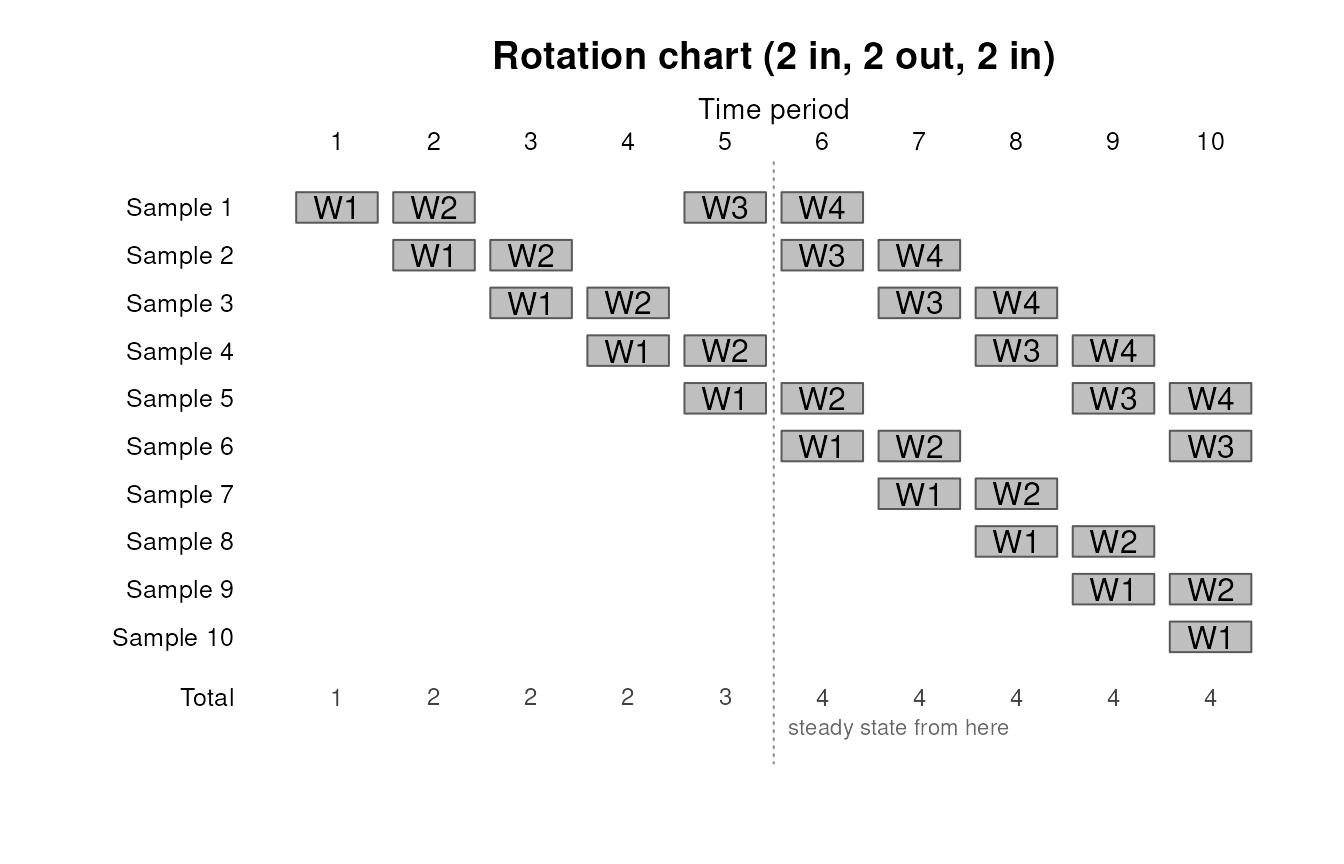

A two-in, two-out, two-in rotation reaches its steady sample at occasion six. The cohort rows show which interviews contribute to overlap between occasions.

design_overlap() describes issued samples. The sizing and power functions define overlap among respondents. They coincide at full response. Otherwise, conversion requires an assumption about response persistence. Under response independent across occasions at rate r, an issued overlap f yields about fr respondent overlap and persistent response moves it closer to f.

Recruit a panel under attrition

n_panel() takes a scalar target from n_prop() or n_mean() and calculates how many units to recruit so enough respondents remain at a target wave. The rates below are illustrative: 72.8% response at recruitment followed by four wave-to-wave retention rates.

target <- n_prop(p = 0.50, moe = 0.031)
panel <- n_panel(
  target,
  retention = c(0.878, 0.963, 0.936, 0.956),
  resp_rate = 0.728
)
panel
#> Panel recruitment (fixed, 5-wave life)
#> issued: 1815 -> 1000 responding at wave 5
#> proportion (wald): se = 0.01582, moe = 0.031, cv = 0.0316
#> 
#>  wave retention n_resp se      moe    
#>  1              1321   0.01376 0.02696
#>  2    0.878     1160   0.01468 0.02878
#>  3    0.963     1117   0.01496 0.02932
#>  4    0.936     1046   0.01546 0.03031
#>  5    0.956     1000   0.01582 0.031  
#> 
#> # summary() for the launch, the loss and per-wave cv
panel$waves[, c("wave", "q", "loss_share", "n_resp", "moe")]
#>   wave         q loss_share    n_resp        moe
#> 1    1 0.7280000 0.60550724 1320.8645 0.02696429
#> 2    2 0.6391840 0.19771592 1159.7190 0.02877675
#> 3    3 0.6155342 0.05264754 1116.8094 0.02932436
#> 4    4 0.5761400 0.08769657 1045.3336 0.03031033
#> 5    5 0.5507898 0.05643274  999.3389 0.03100000

The output reports the units to recruit, expected respondents at each wave, and their expected precision. Initial response and later retention are separate because spreading one average rate across waves changes the required recruitment. The model treats loss as permanent. A study that allows units to return after a missed wave needs a different retention model.

assurance requests a probability of retaining the required responding sample rather than planning only at its expectation:

n_panel(
  target,
  retention = c(0.878, 0.963, 0.936, 0.956),
  resp_rate = 0.728,
  assurance = 0.90
)$n_assured
#> [1] 1865

prec_panel() runs the calculation in the other direction for a recruitment already fixed by budget or operations.

Rotating panels and startup

For a rotating panel, an equal cohort enters each occasion and the estimate combines the live cohorts:

rotating_panel <- n_panel(
  target,
  retention = c(0.878, 0.963, 0.936, 0.956),
  resp_rate = 0.728,
  design = "rotating"
)
c(
  entrants_per_occasion = rotating_panel$n_entrants,
  standing_issue = rotating_panel$n_in_sample
)
#> entrants_per_occasion        standing_issue 
#>              321.3672             1606.8361

n_entrants is the new cohort issued at each mature occasion. n_in_sample is the standing issued sample across all live cohorts. Do not use one as a substitute for the other.

The mature design can start gradually or immediately. A gradual start recruits one cohort per occasion. An immediate start fills the sample on the first occasion with cohorts assigned different remaining participation lengths:

immediate_panel <- n_panel(
  target,
  retention = c(0.878, 0.963, 0.936, 0.956),
  resp_rate = 0.728,
  design = "rotating",
  start = "immediate"
)
immediate_panel$launch[, c("period", "n_in_sample", "n_resp", "moe")]
#>   period n_in_sample    n_resp        moe
#> 1      1    1606.836 1169.7767 0.02865277
#> 2      2    1606.836 1055.6065 0.03016248
#> 3      3    1606.836 1032.8056 0.03049361
#> 4      4    1606.836 1007.4856 0.03087441
#> 5      5    1606.836  999.3389 0.03100000
#> 6      6    1606.836  999.3389 0.03100000

Membership is at its mature level immediately, but response composition is not, because every unit starts at wave 1. $launch_waves shows the wave composition as the design settles.

Build a fieldwork schedule

design_schedule() turns the panel and rotation into an operational manifest without selecting records:

field_plan <- design_schedule(
  immediate_panel,
  rotation = design_rotation("5"),
  horizon = 8,
  horizon_policy = "continuing",
  refreshment = "entrant_register",
  rounding = "ceiling"
)
field_plan
#> Longitudinal design schedule (immediate launch, continuing)
#> life: 5 stages over 8 occasions, steady from occasion 5
#> rounding: ceiling at panel and cohort level
#> issue: 1610 at startup, 322 per occasion (occasions 2-8)
#> tail commitments: 10 panel-interviews after occasion 8
#> # summary() for the occasion-by-occasion profile and the overlap
field_plan$components[, c(
  "cohort", "entry_wave", "operational_issue", "panels", "frame_role"
)]
#>     cohort entry_wave operational_issue panels       frame_role
#> 1  startup          1              1610      5          startup
#> 2 intake_2          2               322      1 entrant_register
#> 3 intake_3          3               322      1 entrant_register
#> 4 intake_4          4               322      1 entrant_register
#> 5 intake_5          5               322      1 entrant_register
#> 6 intake_6          6               322      1 entrant_register
#> 7 intake_7          7               322      1 entrant_register
#> 8 intake_8          8               322      1 entrant_register

The horizon policy states whether interviews promised after the reporting window continue, cohort participation is truncated, or intake closes early. An entrant register assumes later frames contain newly eligible units. A whole-vintage refreshment can also be declared, but the planning object does not infer analysis weights across frame vintages.

The immediate-start chart helps schedule replacement cohorts. It describes issued membership. Use the launch table above for the response composition and precision during startup:

plot(design_overlap(design_rotation("5")), start = "immediate")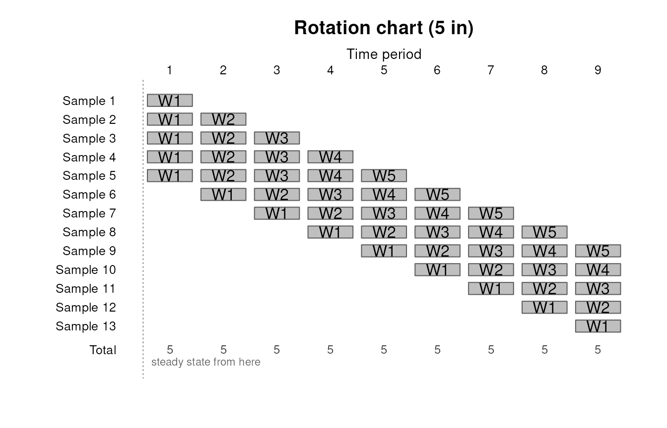

An immediate start fills the issued sample from the first occasion using cohorts with different remaining participation lengths. New cohorts replace departing cohorts over time.

design_rotation() records a rotation already chosen. It does not optimize a pattern for target overlap and respondent burden. Compare candidate patterns by passing their lag-specific overlaps to the precision functions above.

References

U.S. Census Bureau, and U.S. Bureau of Labor Statistics. 2019. Current Population Survey: Design and Methodology. Technical Paper 77. https://www2.census.gov/programs-surveys/cps/methodology/CPS-Tech-Paper-77.pdf.