Precision planning asks how well a survey can estimate one quantity. Power planning asks whether a design can detect a specified difference. State the comparison first, whether two independent groups, two occasions with overlap, or a treated-versus-control change.
The n reported by power_prop() and
power_mean() is the gross sample size per group. For
power_did(), it is the gross sample size per arm per wave.
See Repeated surveys for the
distinction between issued and respondent overlap.
Detect a difference between proportions
How many units per group are needed to detect a change from 70% to 75% with 80% power and a two-sided 5% significance level?
power_prop(
  p1 = 0.70,
  p2 = 0.75,
  power = 0.80,
  alpha = 0.05
)
#> Power analysis for proportions (solved for sample size)
#> n = 1248 (per group), power = 0.800, effect = 0.0500
#> (p1 = 0.700, p2 = 0.750, alpha = 0.05, deff = 1)
Add design and response assumptions in the same units as the sample size:
power_prop(
  p1 = 0.70,
  p2 = 0.75,
  power = 0.80,
  deff = 2,
  resp_rate = 0.85
)
#> Power analysis for proportions (solved for sample size)
#> n = 2937 (net: 2496, per group), power = 0.800, effect = 0.0500
#> (p1 = 0.700, p2 = 0.750, alpha = 0.05, deff = 2.00, resp_rate = 0.85)
The design effect multiplies variance, while the response rate converts the gross issued size into its expected responding size. Neither adjustment addresses nonresponse bias.
Three solve modes
The proportion and mean functions solve for whichever of sample size, power, or effect size is unspecified:
# Gross sample size per group
power_prop(p1 = 0.70, p2 = 0.75, power = 0.80, deff = 2)
#> Power analysis for proportions (solved for sample size)
#> n = 2496 (per group), power = 0.800, effect = 0.0500
#> (p1 = 0.700, p2 = 0.750, alpha = 0.05, deff = 2.00)

# Power at 1,500 issued units per group
power_prop(p1 = 0.70, p2 = 0.75, n = 1500, power = NULL, deff = 2)
#> Power analysis for proportions (solved for power)
#> n = 1500 (per group), power = 0.584, effect = 0.0500
#> (p1 = 0.700, p2 = 0.750, alpha = 0.05, deff = 2.00)

# Minimum detectable second proportion
power_prop(p1 = 0.70, n = 1500, deff = 2)
#> Power analysis for proportions (solved for minimum detectable effect)
#> n = 1500 (per group), power = 0.800, effect = 0.0639
#> (p1 = 0.700, p2 = 0.764, alpha = 0.05, deff = 2.00)
The minimum detectable effect (MDE) is the smallest difference that reaches the requested power under the planning assumptions. A one-sided test changes the critical value and must be justified before looking at results.
For continuous outcomes, supply the anticipated within-group variance:
# Detect a difference of 5 when each group has variance 200
power_mean(var = 200, effect = 5, power = 0.80)
#> Power analysis for means (solved for sample size)
#> n = 126 (per group), power = 0.800, effect = 5.0000
#> (alpha = 0.05, deff = 1)

# MDE at 400 issued units per group
power_mean(var = 200, n = 400)
#> Power analysis for means (solved for minimum detectable effect)
#> n = 400 (per group), power = 0.800, effect = 2.8016
#> (alpha = 0.05, deff = 1)
Unequal groups
ratio is group 1 size divided by group 2 size
(n1 / n2). For example, ratio = 2 allocates
twice as many units to group 1:
power_prop(p1 = 0.30, p2 = 0.35, ratio = 2)
#> Power analysis for proportions (solved for sample size)
#> n1 = 2088, n2 = 1044 (total = 3132), power = 0.800, effect = 0.0500
#> (p1 = 0.300, p2 = 0.350, alpha = 0.05, deff = 1, ratio = 2)
power_mean(var = c(80, 120), effect = 5, ratio = 2)
#> Power analysis for means (solved for sample size)
#> n1 = 101, n2 = 51 (total = 152), power = 0.800, effect = 5.0000
#> (alpha = 0.05, deff = 1, ratio = 2)
When sample sizes are already fixed, supply a length-two
n vector in group 1, group 2 order.
Overlapping occasions
If some respondents are observed at both occasions, their positive outcome correlation reduces the variance of change:
power_prop(
  p1 = 0.70,
  p2 = 0.75,
  power = 0.80,
  deff = 2,
  overlap = 0.50,
  overlap_cor = 0.60
)
#> Power analysis for proportions (solved for sample size)
#> n = 1749 (per group), power = 0.800, effect = 0.0500
#> (p1 = 0.700, p2 = 0.750, alpha = 0.05, deff = 2.00, overlap = 0.50, overlap_cor = 0.60)
overlap is the share of the first occasion’s responding
sample observed again. A rotation object describes issued overlap, so
convert it using an explicit response-persistence assumption when
response is incomplete.
Difference-in-differences
power_did() plans the interaction contrast
(Y_{T,1} - Y_{T,0}) - (Y_{C,1} - Y_{C,0}),
where T and C denote treated and control arms and 0 and 1
denote baseline and endline. Supply each arm as
c(baseline, endline):
# Proportion: treated rises by 5 points while control falls by 2
power_did(
  treat = c(0.50, 0.55),
  control = c(0.50, 0.48),
  outcome = "prop",
  effect = 0.07
)
#> Power analysis for DiD proportions (solved for sample size)
#> n = 1598 (per group), power = 0.800, effect = 0.0700
#> (treat = (0.500, 0.550), control = (0.500, 0.480), alpha = 0.05, deff = 1)

# Mean outcome with half of each arm observed again
power_did(
  treat = c(50, 55),
  control = c(50, 52),
  outcome = "mean",
  var = 100,
  effect = 3,
  overlap = 0.50,
  overlap_cor = 0.60
)
#> Power analysis for DiD means (solved for sample size)
#> n = 245 (per group), power = 0.800, effect = 3.0000
#> (treat = (50.000, 55.000), control = (50.000, 52.000), alpha = 0.05, deff = 1, var = (100.00, 100.00, 100.00, 100.00), overlap = 0.50, overlap_cor = 0.60)
Here n is per arm per wave. Unequal treated and control
arms are supported. Supply n = c(n_treat, n_control) to
evaluate fixed sizes, or ratio = n_treat / n_control when
solving for sizes. Within each arm, the calculation assumes the same
issued size at baseline and endline, and it does not accept four
independently chosen cell sizes.
Alternative proportion methods
Near a boundary, arcsine and log-odds calculations provide transformed-scale alternatives to the untransformed Wald calculation:
power_prop(
  p1 = 0.15,
  p2 = 0.18,
  alternative = "one.sided",
  method = "arcsine"
)
#> Power analysis for proportions (solved for sample size)
#> n = 1890 (per group), power = 0.800, effect = 0.0300
#> (p1 = 0.150, p2 = 0.180, alpha = 0.05, deff = 1, one-sided, method = arcsine)

power_prop(
  p1 = 0.15,
  p2 = 0.18,
  alternative = "one.sided",
  method = "logodds"
)
#> Power analysis for proportions (solved for sample size)
#> n = 1889 (per group), power = 0.800, effect = 0.0300
#> (p1 = 0.150, p2 = 0.180, alpha = 0.05, deff = 1, one-sided, method = logodds)
The methods test differences on different scales and can produce different operating characteristics. Choose the method to match the planned analysis, not after comparing which result is smallest.
Inspect a power curve
The curve shows how many issued units each independent group needs before the design reaches the requested power:
power_plan <- power_prop(
  p1 = 0.70,
  p2 = 0.75,
  power = 0.80,
  deff = 2
)
plot(power_plan)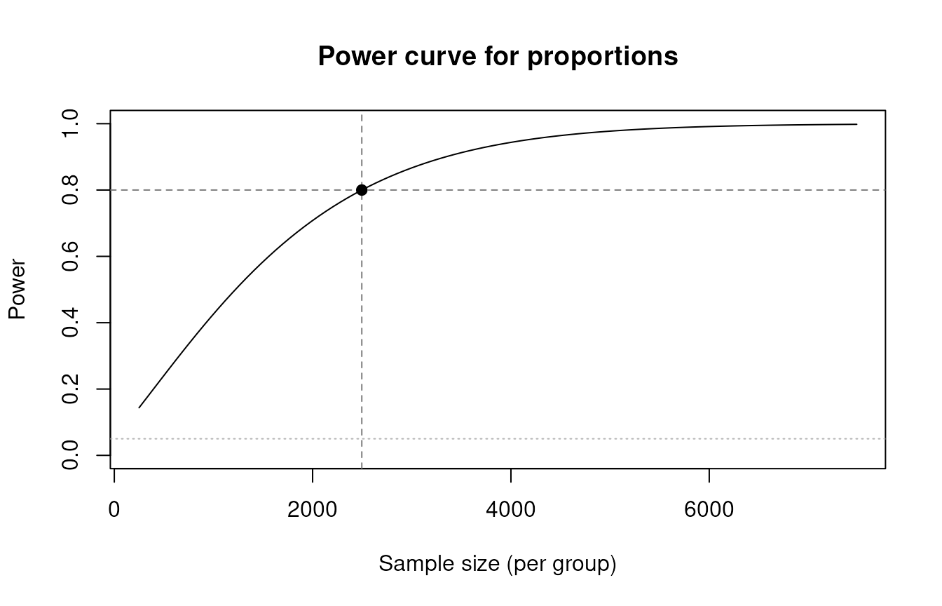
Power to detect a 5 percentage point difference with a design effect of 2 and complete response. The intersection marks the 80 percent power requirement per group.
For exact values, use predict() on supported power
results:
power_at_n <- power_prop(
  p1 = 0.70,
  p2 = 0.75,
  n = 500,
  power = NULL,
  deff = 2
)
predict(power_at_n, data.frame(n = seq(500, 2500, by = 500)))
#>      n     power effect
#> 1  500 0.2407366   0.05
#> 2 1000 0.4260633   0.05
#> 3 1500 0.5839244   0.05
#> 4 2000 0.7081186   0.05
#> 5 2500 0.8006374   0.05
A consistent planning workflow
Suppose the same independent survey design will estimate baseline coverage and compare baseline with a later round. Store shared assumptions once:
design <- svyplan(deff = 2, resp_rate = 0.85)First, size each occasion for a 5 percentage point margin of error and check the expected precision:
occasion <- n_prop(p = 0.70, moe = 0.05, plan = design)
occasion
#> Sample size for proportion (wald)
#> n = 760 gross (net: 646) (p = 0.70, moe = 0.050, deff = 2.00, resp_rate = 0.85)
#> expected cases = 451.8
prec_prop(occasion)
#> Sampling precision for proportion (wald)
#> n = 760 (net: 646)
#> se = 0.0255, moe = 0.0500, cv = 0.0364, rmoe = 0.0714
#> expected cases = 451.8
Then evaluate the power to detect a change from 70% to 75% when both occasions issue that many units:
power_prop(
  p1 = 0.70,
  p2 = 0.75,
  n = as.integer(occasion),
  power = NULL,
  plan = design
)
#> Power analysis for proportions (solved for power)
#> n = 760 (net: 646, per group), power = 0.297, effect = 0.0500
#> (p1 = 0.700, p2 = 0.750, alpha = 0.05, deff = 2.00, resp_rate = 0.85)
If that power is insufficient, solve for the per-occasion requirement and use the larger of the precision and power sizes:
power_requirement <- power_prop(
  p1 = 0.70,
  p2 = 0.75,
  power = 0.80,
  plan = design
)

max(
  precision = as.integer(occasion),
  power = as.integer(power_requirement)
)
#> [1] 2937
The design effect and response rate are planning guesses. Check how the power requirement moves across plausible values before fixing the sample:
predict(
  power_requirement,
  expand.grid(
    deff = c(1.5, 2.0, 2.5),
    resp_rate = c(0.75, 0.85, 0.95)
  )
)
#>   deff resp_rate        n power effect
#> 1  1.5      0.75 2495.938   0.8   0.05
#> 2  2.0      0.75 3327.917   0.8   0.05
#> 3  2.5      0.75 4159.896   0.8   0.05
#> 4  1.5      0.85 2202.298   0.8   0.05
#> 5  2.0      0.85 2936.397   0.8   0.05
#> 6  2.5      0.85 3670.497   0.8   0.05
#> 7  1.5      0.95 1970.477   0.8   0.05
#> 8  2.0      0.95 2627.303   0.8   0.05
#> 9  2.5      0.95 3284.128   0.8   0.05
The requirement is proportional to the design effect and inversely proportional to the response rate, so the grid brackets the sample the field budget must cover.
Meeting a precision target does not automatically meet a power target. This workflow keeps the design effect, response rate, sample-size units, and group definition consistent across both calculations. Surveys with several indicators combine their requirements as shown in Multiple indicators and domains. A clustered design uses variance components and stage costs in place of the scalar design effect, as in Multistage survey planning, and a stratified design adds the steps in Stratification and sample allocation.