Survey sample size determination, precision analysis, optimal allocation, stratification, and power analysis for R.
Sample sizes
library(svyplan)

# Proportion with margin of error
n_prop(p = 0.3, moe = 0.05)
#> Sample size for proportion (wald)
#> n = 323 (p = 0.30, moe = 0.050)

# Mean with finite population and design effect
n_mean(var = 100, moe = 2, N = 5000, deff = 1.5)
#> Sample size for mean
#> n = 141 (var = 100.00, moe = 2.000, deff = 1.50)
Response rate adjustment
Most sizing and precision functions accept resp_rate. In sample-size mode, the required sample is inflated by 1 / resp_rate to account for expected non-response:
n_prop(p = 0.3, moe = 0.05, deff = 1.5, resp_rate = 0.8)
#> Sample size for proportion (wald)
#> n = 606 (net: 485) (p = 0.30, moe = 0.050, deff = 1.50, resp_rate = 0.80)
Survey plan profiles
When the same design parameters apply across many calls, bundle them into a svyplan() profile:
plan <- svyplan(deff = 1.5, resp_rate = 0.85, N = 50000)

# Pass as argument
n_prop(p = 0.3, moe = 0.05, plan = plan)
#> Sample size for proportion (wald)
#> n = 564 (net: 480) (p = 0.30, moe = 0.050, deff = 1.50, resp_rate = 0.85)

# Or pipe (positional or named args)
plan |> n_mean(100, moe = 2)
#> Sample size for mean
#> n = 169 (net: 144) (var = 100.00, moe = 2.000, deff = 1.50, resp_rate = 0.85)
plan |> n_mean(var = 100, moe = 2)
#> Sample size for mean
#> n = 169 (net: 144) (var = 100.00, moe = 2.000, deff = 1.50, resp_rate = 0.85)

# Explicit args always override plan defaults
n_prop(p = 0.3, moe = 0.05, plan = plan, deff = 2.0)
#> Sample size for proportion (wald)
#> n = 750 (net: 638) (p = 0.30, moe = 0.050, deff = 2.00, resp_rate = 0.85)
Precision analysis
Given a sample size, how precise will your estimates be? The prec_*() functions are the inverse of n_*():
prec_prop(p = 0.3, n = 400)
#> Sampling precision for proportion (wald)
#> n = 400
#> se = 0.0229, moe = 0.0449, cv = 0.0764

prec_mean(var = 100, n = 400, mu = 50)
#> Sampling precision for mean
#> n = 400
#> se = 0.5000, moe = 0.9800, cv = 0.0100
Round-trip between size and precision
All n_*() and prec_*() functions are S3 generics. Pass a precision result to n_*() to recover the sample size, or pass a sample size result to prec_*() to compute the achieved precision:
# Start with a precision target
s <- n_prop(p = 0.3, moe = 0.05, deff = 1.5)

# What precision does this n achieve?
p <- prec_prop(s)
p
#> Sampling precision for proportion (wald)
#> n = 485
#> se = 0.0255, moe = 0.0500, cv = 0.0850

# Recover the original n
n_prop(p)
#> Sample size for proportion (wald)
#> n = 485 (p = 0.30, moe = 0.050, deff = 1.50)
Multi-indicator surveys
Household surveys track many indicators at once. n_multi() finds the sample size that satisfies all precision targets simultaneously.
targets <- data.frame(
  name = c("stunting", "vaccination", "anemia"),
  p    = c(0.25, 0.70, 0.12),
  moe  = c(0.05, 0.05, 0.03),
  deff = c(2.0, 1.5, 2.5)
)

n_multi(targets)
#> Multi-indicator sample size
#> n = 1127 (binding: anemia)
#> ---
#>  name        .n   .cv_target .cv_achieved .binding
#>  stunting     577 0.10204269 0.07297042
#>  vaccination  485 0.03644382 0.02388518
#>  anemia      1127 0.12755336 0.12755336   *
Per-domain optimization works by specifying domain columns via the domains parameter.
MICS/DHS-style relative margin of error
Programmes like UNICEF MICS and DHS express precision as a relative margin of error (RME = MOE / p). To use this with svyplan, convert to an absolute margin of error: moe = RME * p.
# RME = 12% for each indicator
rme <- 0.12
targets_rme <- data.frame(
  name = c("stunting", "vaccination", "anemia"),
  p    = c(0.25, 0.70, 0.12),
  deff = c(2.0, 1.5, 2.5)
)
targets_rme$moe <- rme * targets_rme$p

n_multi(targets_rme)
#> Multi-indicator sample size
#> n = 4891 (binding: anemia)
#> ---
#>  name        .n   .cv_target .cv_achieved .binding
#>  stunting    1601 0.06122561 0.03502580
#>  vaccination  172 0.06122561 0.01146488
#>  anemia      4891 0.06122561 0.06122561   *
The MICS template reports sample size in households. svyplan returns the number of individuals in the target population. To convert, divide by the expected number of eligible individuals per household: n_hh = ceiling(n / (pb * hh_size)), where pb is the share of the target population and hh_size is the average household size.
Multistage cluster designs
# Optimal 2-stage allocation within a budget
n_cluster(stage_cost = c(500, 50), delta = 0.05, budget = 100000)
#> Optimal 2-stage allocation
#> field design: n_psu = 80 | psu_size = 15 -> total n = 1200
#> cv = 0.0376, cost = 100000
#> continuous optimum: n_psu = 84.08997 | psu_size = 13.78405 (cv = 0.0376, cost = 100000)

# Precision for a given allocation
prec_cluster(n = c(50, 12), delta = 0.05)
#> Sampling precision for 2-stage cluster
#> n_psu = 50 | psu_size = 12 -> total n = 600
#> cv = 0.0508
Variance components can be estimated from frame data and passed directly to n_cluster():
set.seed(104)
frame <- data.frame(
  district = rep(1:40, each = 20),
  income = rep(rnorm(40, 500, 100), each = 20) + rnorm(800, 0, 50)
)

vc <- varcomp(income ~ district, data = frame)
vc
#> Variance components (2-stage)
#> varb = 0.0255, varw = 0.0099
#> delta = 0.7210
#> k = 1.0317
#> Unit relvariance = 0.0343
as.data.frame(vc)
#>   stages       varb        varw     delta       k   rel_var
#> 1      2 0.02554834 0.009886668 0.7209915 1.03174 0.0343449

n_cluster(stage_cost = c(500, 50), delta = vc, cv = 0.05)
#> Optimal 2-stage allocation
#> field design: n_psu = 13 | psu_size = 2 -> total n = 26
#> cv = 0.0484, cost = 7800
#> continuous optimum: n_psu = 12.22966 | psu_size = 1.967178 (cv = 0.0500, cost = 7318)
delta is the survey-planning measure of homogeneity used by varcomp(), n_cluster(), and design_effect(). It is not the same as a generic mixed-model ICC, and values near 0 or 1 correspond to degenerate boundary cases for the closed-form cluster optimizer.
Sensitivity analysis
predict() evaluates a result at new parameter combinations, returning a data frame suitable for plotting:
x <- n_prop(p = 0.3, moe = 0.05, deff = 1.5)
predict(x, expand.grid(
  deff = c(1, 1.5, 2, 2.5),
  resp_rate = c(0.7, 0.8, 0.9, 1.0)
))
#>    deff resp_rate         n         se  moe         cv
#> 1   1.0       0.7  460.9751 0.02551067 0.05 0.08503558
#> 2   1.5       0.7  691.4626 0.02551067 0.05 0.08503558
#> 3   2.0       0.7  921.9501 0.02551067 0.05 0.08503558
#> 4   2.5       0.7 1152.4376 0.02551067 0.05 0.08503558
#> 5   1.0       0.8  403.3532 0.02551067 0.05 0.08503558
#> 6   1.5       0.8  605.0298 0.02551067 0.05 0.08503558
#> 7   2.0       0.8  806.7064 0.02551067 0.05 0.08503558
#> 8   2.5       0.8 1008.3829 0.02551067 0.05 0.08503558
#> 9   1.0       0.9  358.5362 0.02551067 0.05 0.08503558
#> 10  1.5       0.9  537.8042 0.02551067 0.05 0.08503558
#> 11  2.0       0.9  717.0723 0.02551067 0.05 0.08503558
#> 12  2.5       0.9  896.3404 0.02551067 0.05 0.08503558
#> 13  1.0       1.0  322.6825 0.02551067 0.05 0.08503558
#> 14  1.5       1.0  484.0238 0.02551067 0.05 0.08503558
#> 15  2.0       1.0  645.3651 0.02551067 0.05 0.08503558
#> 16  2.5       1.0  806.7064 0.02551067 0.05 0.08503558
Sensitivity analysis is available for single-indicator sample-size and precision results, cluster designs, power analyses, and strata boundaries. Multi-indicator results are not currently supported by predict().
Strata boundaries
strata_bound() finds optimal boundaries for a continuous stratification variable.
set.seed(905)
x <- rlnorm(5000, meanlog = 6, sdlog = 1.2)

strata_bound(x, n_strata = 4, n = 300, method = "cumrootf")
#> Strata boundaries (Dalenius-Hodges, 4 strata)
#> Boundaries: 400.0, 1300.0, 3200.0
#> n = 300, cv = 0.0205
#> Allocation: neyman
#> ---
#>  stratum lower       upper    N    share sd     n
#>  1          8.380438   400.00 2492 0.498 104.2   46
#>  2        400.000000  1300.00 1647 0.329 246.5   71
#>  3       1300.000000  3200.00  639 0.128 500.9   56
#>  4       3200.000000 28909.53  222 0.044 3264.3 127
Four methods are available: Dalenius-Hodges ("cumrootf"), geometric ("geo"), Lavallée-Hidiroglou ("lh"), and Kozak ("kozak").
Power analysis
Solve for sample size, power, or minimum detectable effect. Supports design effects, finite population correction, response rate adjustment, panel overlap, unequal groups, and allocation ratios. Arcsine and log-odds methods available for rare proportions.
# Sample size to detect a 5pp change from 70% with deff = 2
power_prop(p1 = 0.70, p2 = 0.75, deff = 2.0)
#> Power analysis for proportions (solved for sample size)
#> n = 2496 (per group), power = 0.800, effect = 0.0500
#> (p1 = 0.700, p2 = 0.750, alpha = 0.05, deff = 2.00)

# MDE with n = 1500 per group
power_prop(p1 = 0.70, n = 1500, deff = 2.0)
#> Power analysis for proportions (solved for minimum detectable effect)
#> n = 1500 (per group), power = 0.800, effect = 0.0639
#> (p1 = 0.700, p2 = 0.764, alpha = 0.05, deff = 2.00)

# Means
power_mean(200, effect = 5)
#> Power analysis for means (solved for sample size)
#> n = 126 (per group), power = 0.800, effect = 5.0000
#> (alpha = 0.05)

# Arcsine method for rare proportions
power_prop(p1 = 0.15, p2 = 0.18, alternative = "one.sided",
           method = "arcsine")
#> Power analysis for proportions (solved for sample size)
#> n = 1890 (per group), power = 0.800, effect = 0.0300
#> (p1 = 0.150, p2 = 0.180, alpha = 0.05, one-sided, method = arcsine)

# Difference-in-differences
power_did(treat = c(0.50, 0.55), control = c(0.50, 0.48),
          outcome = "prop", effect = 0.07)
#> Power analysis for DiD proportions (solved for sample size)
#> n = 1598 (per group), power = 0.800, effect = 0.0700
#> (treat = (0.500, 0.550), control = (0.500, 0.480), alpha = 0.05)
plot() draws the power-vs-sample-size curve with reference lines at the solved point:
pw <- power_prop(p1 = 0.70, p2 = 0.75, power = 0.80, deff = 2.0)
plot(pw)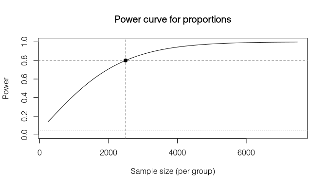
Stratified allocation
Given a sampling frame with stratum sizes and variabilities, n_alloc() distributes the total sample across strata:
frame <- data.frame(
  N = c(4000, 3000, 3000),
  sd = c(10, 15, 8),
  mean = c(50, 60, 55)
)

n_alloc(frame, n = 600, alloc = "neyman")
#> Stratum allocation (neyman, 3 strata)
#> field design: n = 600, cv = 0.0079, cost = 600
#> continuous optimum: n = 600, cv = 0.0079, se = 0.4305
Constraints and alternative solve modes are also supported:
frame_constraints <- transform(
  frame,
  unit_cost = c(1, 1.5, 1),
  max_weight = c(25, 20, NA),
  take_all = c(FALSE, FALSE, TRUE)
)

# Budget-constrained allocation with weight and take-all constraints
n_alloc(frame_constraints, budget = 3500, alloc = "optimal", min_n = 40)
#> Stratum allocation (optimal, 3 strata)
#> field design: n = 3403, cv = 0.0076, cost = 3500
#> continuous optimum: n = 3403.425, cv = 0.0076, se = 0.4125
#> (min_n = 40)
Domain-level CV targets can be enforced via the domains parameter:
frame_domains <- data.frame(
  province = c("North", "North", "South", "South"),
  stratum = c("Urban", "Rural", "Urban", "Rural"),
  N = c(2000, 3000, 1800, 3200),
  sd = c(12, 18, 10, 16),
  mean = c(55, 48, 58, 50)
)

# Minimum total n such that each province meets the CV target
n_alloc(frame_domains, domains = "province",
        cv = 0.04, alloc = "power", power_q = 0.3)
#> Stratum allocation (power, 4 strata)
#> field design: n = 112, cv = 0.0270, cost = 112
#> continuous optimum: n = 110.7422, cv = 0.0272, se = 1.4076
#> Domains: 2
#> ---
#>  province .domain .n       .se      .moe     .cv    .cost
#>  North    5_North 59.23404 2.032000 3.982647 0.0400 59
#>  South    5_South 51.50815 1.948447 3.818886 0.0368 52
prec_alloc() computes the precision for a given allocation (inverse of n_alloc()).
Adding a delta_psu column to the frame (for example from varcomp() with its strata argument) turns the allocation into a stratified two-stage design, with cost-optimal or fixed cluster takes per stratum. See ?n_alloc and the vignette for the full workflow.
Design effects
# Planning: expected cluster design effect
design_effect(delta = 0.05, psu_size = 20, method = "cluster")
#> Design effect (Cluster)
#> overall = 1.9500

# Diagnostic: Kish design effect from weights
set.seed(2718)
w <- runif(500, 0.5, 4)
design_effect(w, method = "kish")
#> Design effect (Kish)
#> overall = 1.1867
effective_n(w, method = "kish")
#> [1] 421.3472