Sample overlap a rotation schedule produces

Compute the fraction of the units a rotation schedule puts in sample that it carries from one occasion to another, at every lag the schedule reaches. This is the overlap of the issued sample, a property of the schedule alone. It is the overlap that n_change(), prec_change(), power_mean(), power_prop() and power_did() take when response is complete, replacing a number the planner would otherwise have to know. See Details for what a response rate below 1 does to that reading.

Usage

design_overlap(schedule, max_lag = NULL)

Arguments

schedule

The occasions a unit spends in and out of sample over its whole life, in one of two forms.

A compact string in either of the two notations the literature uses, told apart by whether it contains a 0. Without one it names the spells in order, starting in sample: "4-8-4" is the CPS pattern, four occasions in, eight out, four in, and "5" is a five-occasion panel with no break. The count of spells must be odd, so the life starts and ends in sample. With a 0 it is one flag per occasion: "1-1-0-0-1-1" is in for two, out for two, in for two, the same life as "2-2-2". A string of all 1s is the one form both notations claim and is refused, naming the two readings and the unambiguous spelling of each.

A numeric or logical vector gives one entry per occasion of a unit's life, 0/FALSE for out of sample. Positive values may differ, in which case they are the number of units still measured at that occasion of the life, which is how a design that subsamples later waves is described. No entry may exceed the first, a wave being able only to re-interview part of the cohort it recruited. The first and last entries must be positive, since an out-of-sample spell before the first or after the last interview is not part of a unit's life. A life shorter than two occasions is refused, having no lag at which any sample is shared.

max_lag

Largest lag to report. Defaults to one less than the life, which is the largest lag at which any overlap is possible.

Value

A svyplan_overlap object: a numeric vector of issued-sample overlap fractions named by lag, so x[1] is the consecutive-occasion overlap and x[12] the overlap a year apart on monthly occasions. Subsetting returns a plain number, which is what the overlap arguments take, and arithmetic returns bare numerics. It also carries:

$shared: Units in sample on both occasions, at each lag.
$n_occasion: Units in sample at any one occasion. Constant, see Details.
$schedule: The resolved per-occasion vector.
$life: Occasions from a unit's first interview to its last.

Details

One cohort enters at every occasion, so at a steady state the cohorts alive span every stage of the life and the sample at occasion $t$ is $\sum_s w_s$, writing $w$ for the schedule. Units in sample at both $t$ and $t + m$ are those whose cohort is in sample at stages $s$ and $s + m$, so

$$\mathrm{shared}(m) = \sum_{s = 1}^{L - m} \min(w_s, w_{s + m}), \qquad \mathrm{overlap}(m) = \mathrm{shared}(m) / \sum_s w_s.$$

The min is the count when the smaller take at the two occasions is a subset of the larger, which is what attrition and planned subsampling both give, including a design that subsamples an interim wave and returns to the whole cohort afterwards. Nesting is an assumption about the design and is not identifiable from the takes. Where the two occasions measure partly disjoint subsamples of the cohort, min is the largest overlap the takes admit rather than the overlap the design has.

These are the overlaps of the design at a steady state, which a rotation reaches once every stage of the life is represented at one occasion. Which occasion that is depends on how the design is launched, and the overlaps themselves do not: shared(m) sums over stages, and entry dates do not enter it. A design that recruits one cohort an occasion reaches the steady state at the occasion that spans the life, the overlaps before it being those of a design no cohort has yet aged out of. A design whose first occasion contains launch components for every possible remaining life length is at the steady state from the first occasion, and these figures hold throughout. For an unbroken equal-take life, those are equal panels planned for lives from the full life down to one occasion, all at their first interview.

Covering every stage is the exact requirement, and for a life with a gap it is more than one cohort per remaining length. Under "1-1-0-0-1-1" the stages that hold the steady state include two that are out of sample, so the cohorts starting there are selected but not interviewed until they reach their first in-sample stage. Splitting the first occasion's interviewed sample alone puts six cohorts in sample where the design holds four, and gives a consecutive overlap of 0.83 against the schedule's 0.50. 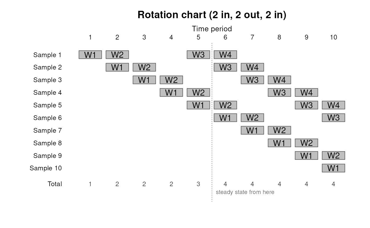plot.svyplan_overlap() draws the one-cohort-an-occasion launch and marks the occasion the steady state begins.

The overlap has one direction here, and that is a property of the steady state rather than a simplification. Elsewhere in the package overlap is n12 / n1 and is not symmetric when the occasions differ in size. Under a stationary rotation every occasion holds the same mix of life stages, so $n_t$ is the same at every occasion and the two directions coincide. A design whose cohorts differ in size by entry date has no steady state and is outside what this function describes.

Why a life, and not a repeating pattern

A schedule is a finite life, not a cycle. Reading "4-8-4" as "four in, eight out, repeat forever" gives the wrong answer, and gives it quietly. Under the cycle only the cohort finishing its four-occasion stint leaves each occasion, so seven of eight are retained and the consecutive overlap comes out at 87.5%. Under the finite life two cohorts leave, one reaching the end of its first spell and one reaching the end of its second, so six of eight are retained and the answer is the published 75%. A compact string with an even number of spells would have to be read as a cycle and is rejected for that reason.

Two notations, and the one string that means both

Rotation designs are named two ways in print. "4-8-4" counts occasions per spell; "1-1-0-0-1-1" carries one flag per occasion. Both are accepted, told apart by the 0, which no spell can be. The exception is a string of all 1s, which is a valid sentence in both notations and a different design in each: "1-1-1" is three occasions in sample as a pattern and one in, one out, one in as spells, whose consecutive overlaps are 2/3 and 0. Neither reading is given precedence, because the wrong one is invisible in the answer. Write "3" or "1-0-1", which each say one thing only.

Issued overlap, and the overlap a variance formula reads

What a schedule fixes is which units are issued at both occasions. The overlap argument of n_change(), prec_change() and the power family is the fraction of the first occasion's responding sample measured again, those functions netting each occasion down by resp_rate before the covariance forms. The two are the same number at resp_rate = 1, and this function's result can be passed straight through there.

Below full response they are not, and converting one into the other needs an assumption about how response persists across occasions, which neither function makes. Under response independent between occasions at rate $r$, an issued overlap $f$ leaves a responding overlap of about $fr$: a shared unit responds at both occasions with probability $r^2$, against the $r$ of issued units responding at the first. A panel whose wave-1 respondents are much likelier to respond again sits above that, reaching $f$ itself when response persists perfectly. Pass the figure you expect among respondents, and say which assumption produced it.

What it does not give you

The correlation between occasions. overlap is a property of the schedule and is fixed once the design is declared; overlap_cor is a property of the variable being measured and has to come from a previous round of the same survey. Both enter the variance of a change, and only their product buys precision, so a schedule alone does not say what a rotation is worth.

References

U.S. Census Bureau. Current Population Survey: Design and Methodology, Technical Paper 77. The 4-8-4 rotation and its 75% and 50% overlaps.

Lynn, P. (2012). Longitudinal Survey Methods for the Household Finance and Consumption Survey. Report to the European Central Bank. The one-flag-per-occasion notation, and the 1-1-0-0-1-1 design whose lag profile the examples reproduce.

Examples

# CPS 4-8-4: 75 percent month to month, 50 percent a year apart
cps <- design_overlap("4-8-4")
cps[1]
#> [1] 0.75
cps[12]
#> [1] 0.5

# A five-wave panel with no break
design_overlap("5")[1]
#> [1] 0.8

# Feed it straight into a change requirement, response being complete here
n_change(p = c(0.30, 0.36), moe = 0.02,
         overlap = cps[1], overlap_cor = 0.5)
#> Sample size for change (proportion scale)
#> n = 2646 per occasion (p = 0.3 to 0.36, moe = 0.02, deff = 1)
#> overlap = 0.75, overlap_cor = 0.5 (62.5% of the independent variance)

# The annual lag is the one a year-on-year change uses
n_change(p = c(0.30, 0.36), moe = 0.02,
         overlap = cps[12], overlap_cor = 0.5)
#> Sample size for change (proportion scale)
#> n = 3174 per occasion (p = 0.3 to 0.36, moe = 0.02, deff = 1)
#> overlap = 0.5, overlap_cor = 0.5 (75.0% of the independent variance)

# Under response independent between occasions at 80 percent, the overlap
# among respondents is the issued one scaled by the response rate
n_change(p = c(0.30, 0.36), moe = 0.02, resp_rate = 0.8,
         overlap = cps[1] * 0.8, overlap_cor = 0.5)
#> Sample size for change (proportion scale)
#> n = 3703 per occasion (net: 2962) (p = 0.3 to 0.36, moe = 0.02, deff = 1, resp_rate = 0.80)
#> overlap = 0.6, overlap_cor = 0.5 (70.0% of the independent variance)

# One flag per occasion, the other notation in use: in for two, out for
# two, in for two. Change is estimable at lags 1, 3, 4 and 5 but not 2
design_overlap("1-1-0-0-1-1")
#> Rotation overlap (planning)
#> 
#>   6-occasion life, 4 in sample each occasion
#>   schedule: 2 in, 2 out, 2 in
#> 
#>  lag shared overlap
#>  1   2      0.5    
#>  2   0      0      
#>  3   1      0.25   
#>  4   2      0.5    
#>  5   1      0.25   

# The same design as spell lengths
identical(as.double(design_overlap("2-2-2")),
          as.double(design_overlap("1-1-0-0-1-1")))
#> [1] TRUE

# An explicit schedule, halving the take at later waves
design_overlap(c(1, 1, 0.5, 0.5))
#> Rotation overlap (planning)
#> 
#>   4-occasion life, 3 in sample each occasion
#>   schedule: 2 in, 2 in at 0.5
#> 
#>  lag shared overlap
#>  1   2.0    0.6667 
#>  2   1.0    0.3333 
#>  3   0.5    0.1667 

# The chart of the schedule, one row per cohort
plot(design_overlap("1-1-0-0-1-1"))