Survey sample size planning with svyplan

svyplan provides a toolkit for survey sample size determination. It covers sample sizes for proportions and means, precision analysis, multistage cluster allocation, multi-indicator optimization, strata boundary optimization, and power analysis. The core sizing and precision functions use paired S3 interfaces for round-trip conversions. Sensitivity analysis via predict() is available for supported result classes.

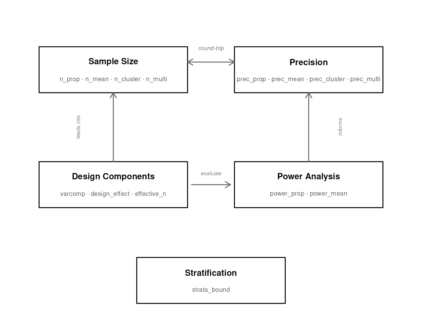
Function ecosystem

The package exports 31 functions organized into six families. The diagram below shows how they relate to each other.

Family	Functions	Purpose
Plan	svyplan	Reusable profile for design defaults
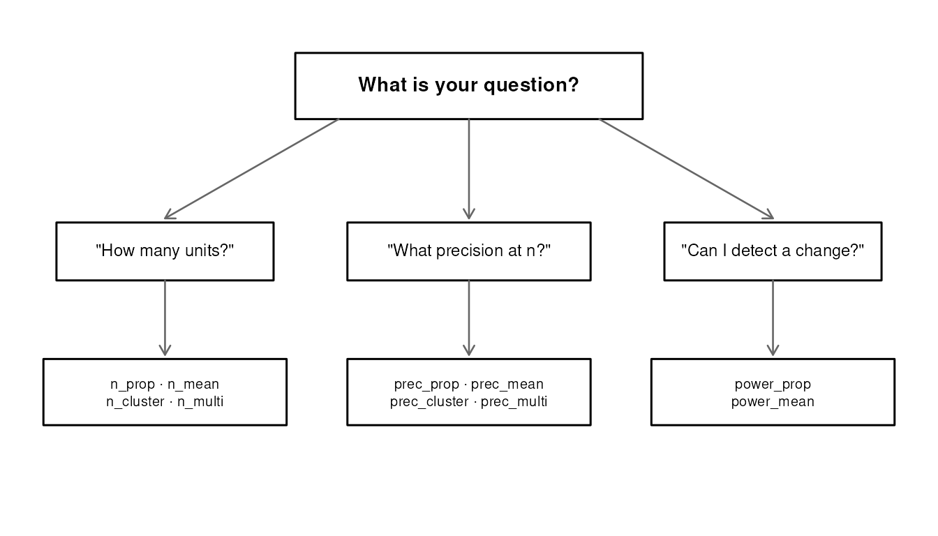
Sample size	n_prop, n_mean, n_cluster, n_multi, n_multi_cluster, n_alloc, n_twophase, n_change, n_panel, n_pooled	“How many units do I need?”
Precision	prec_prop, prec_mean, prec_cluster, prec_multi, prec_multi_cluster, prec_alloc, prec_twophase, prec_change, prec_panel, prec_pooled	“What precision does n achieve?”
Power	power_prop, power_mean, power_did	“Can I detect a difference?”
Design	varcomp, design_effect, effective_n, design_df, design_overlap, design_schedule	Variance components, design effects, degrees of freedom, and rotation schedules
Strata	strata_bound	Optimal stratification boundaries

The same table read by question rather than by family, since several questions cut across the rows:

Question	Where
How many units for a target precision on a level?	n_prop, n_mean, and the cluster, allocation and two-phase members
How many for a target precision on a change between two occasions?	n_change
How many to recruit so that enough survive to a later wave?	n_panel
How many for a target precision on an average across occasions, an annual figure from quarterly rounds?	n_pooled
What precision does a design I already have achieve?	the prec_* counterpart of each
Can I detect a difference, and how large a one?	power_prop, power_mean, power_did
Can I detect a change over two occasions?	power_prop and power_mean with overlap set, which is the same variance n_change inverts
What overlap does my rotation schedule produce?	design_overlap
What should each startup or intake cohort issue, and when is it active?	design_schedule
What design effect, effective size or degrees of freedom will the design have?	design_effect, effective_n, design_df, varcomp

Most planning functions return structured S3 objects. Available methods depend on the result class; see the relevant help page for details.

The n_*/prec_* duality

The most distinctive feature of svyplan is the bidirectional link between sample size and precision functions. Every n_* function has a prec_* counterpart, and each pair supports round-trip conversion. Under the same formula and continuous design assumptions, converting a result to its counterpart and back reproduces the original target. Changing methods or using an operational integer allocation can change the result.

Because n_* and prec_* are S3 generics, you can pass a result object directly to its inverse. All design parameters travel with the object:

# Compute sample size for a proportion
s <- n_prop(p = 0.3, moe = 0.05, deff = 1.5)
s
#> Sample size for proportion (wald)
#> n = 485 (p = 0.30, moe = 0.050, deff = 1.50)
#> expected cases = 145.2

# What precision does this n achieve?
p <- prec_prop(s)
p
#> Sampling precision for proportion (wald)
#> n = 485
#> se = 0.0255, moe = 0.0500, cv = 0.0850, rmoe = 0.1667
#> expected cases = 145.2

# Recover the original sample size
n_prop(p)
#> Sample size for proportion (wald)
#> n = 485 (p = 0.30, moe = 0.050, deff = 1.50)
#> expected cases = 145.2

You can also override a parameter on the way back:

n_prop(p, cv = 0.08)
#> Sample size for proportion (wald)
#> n = 547 (p = 0.30, cv = 0.080, deff = 1.50)
#> expected cases = 164.1

Sample sizes for proportions and means

Proportions

Estimate vaccination coverage (expected ~70%) with a 5 percentage point margin of error:

n_prop(p = 0.70, moe = 0.05)
#> Sample size for proportion (wald)
#> n = 323 (p = 0.70, moe = 0.050, deff = 1)
#> expected cases = 225.9

Four method options control how the margin of error is computed:

• "wald" (default): the textbook normal approximation
• "wilson": Wilson score interval, better coverage near 0 or 1
• "logodds": log-odds transformation, the right choice when the plan will be reported as an odds ratio
• "beta": Korn-Graubard interval, for a proportion whose expected number of positive counts is small. It stays inside $[0, 1]$ by construction, and a df argument widens it for a variance estimated from few clusters.

n_prop(p = 0.05, moe = 0.02, method = "wald")
#> Sample size for proportion (wald)
#> n = 457 (p = 0.05, moe = 0.020, deff = 1)
#> expected cases = 22.8
n_prop(p = 0.05, moe = 0.02, method = "wilson")
#> Sample size for proportion (wilson)
#> n = 469 (p = 0.05, moe = 0.020, deff = 1)
#> expected cases = 23.4
n_prop(p = 0.05, moe = 0.02, method = "logodds")
#> Sample size for proportion (logodds)
#> n = 475 (p = 0.05, moe = 0.020, deff = 1)
#> expected cases = 23.7
n_prop(p = 0.05, moe = 0.02, method = "beta", df = 25)
#> Sample size for proportion (beta)
#> n = 558 (p = 0.05, moe = 0.020, deff = 1)
#> expected cases = 27.9

The four differ materially only when the expected count is small. For sizing that difference is rarely worth acting on; for assessing an achieved design it often is. ?n_prop has the full comparison.

Target a coefficient of variation instead of a margin of error:

n_prop(p = 0.70, cv = 0.05)
#> Sample size for proportion (wald)
#> n = 172 (p = 0.70, cv = 0.050, deff = 1)
#> expected cases = 120.0

Or state the margin of error as a fraction of the proportion rather than in percentage points. rmoe = 0.07 at p = 0.70 asks for the same interval as moe = 0.049, and says it in the units MICS and DHS state a requirement in:

n_prop(p = 0.70, rmoe = 0.07)
#> Sample size for proportion (wald)
#> n = 336 (p = 0.70, rmoe = 0.070, deff = 1)
#> expected cases = 235.2

The three are targets on one design, not three designs. moe and rmoe fix the interval the chosen method builds, cv fixes the sampling variance underneath it, and every result reports all of them back whichever one you supplied.

Means

Estimate average household expenditure (variance = 40,000, mean = 800) with a margin of error of 30:

n_mean(var = 40000, moe = 30)
#> Sample size for mean
#> n = 171 (var = 40000.00, moe = 30.000, deff = 1)

Common parameters

Most single-stage n_*() and prec_*() functions share these parameters:

Parameter	Meaning
deff	Design effect multiplier (default 1)
N	Finite population size (enables FPC correction)
alpha	Significance level (default 0.05)
resp_rate	Expected response rate (inflates n by 1/resp_rate)

n_prop(p = 0.70, moe = 0.05, deff = 1.5, N = 50000, resp_rate = 0.85)
#> Sample size for proportion (wald)
#> n = 564 gross (net: 480) (p = 0.70, moe = 0.050, deff = 1.50, resp_rate = 0.85)
#> expected cases = 335.6

The design effect can be less than 1 for efficient designs (e.g. well-stratified or PPS samples). svyplan accepts any deff > 0.

n_cluster() / prec_cluster() use cluster-specific inputs instead (stage_cost, icc, unit_relvar, and optionally resp_rate_psu), and n_alloc() / prec_alloc() have their own allocation-oriented interfaces.

Survey plan profiles

When the same deff, N, resp_rate, or alpha apply across many single-stage calls, bundle them into a svyplan() profile to avoid repetition:

plan <- svyplan(deff = 1.5, resp_rate = 0.85, N = 50000)

# Pass as a named argument
n_prop(p = 0.3, moe = 0.05, plan = plan)
#> Sample size for proportion (wald)
#> n = 564 gross (net: 480) (p = 0.30, moe = 0.050, deff = 1.50, resp_rate = 0.85)
#> expected cases = 143.8
n_mean(var = 100, moe = 2, plan = plan)
#> Sample size for mean
#> n = 169 gross (net: 144) (var = 100.00, moe = 2.000, deff = 1.50, resp_rate = 0.85)
power_prop(p1 = 0.30, p2 = 0.35, plan = plan)
#> Power analysis for proportions (solved for sample size)
#> n = 2328 (net: 1979, per group), power = 0.800, effect = 0.0500
#> (p1 = 0.300, p2 = 0.350, alpha = 0.05, deff = 1.50, resp_rate = 0.85)

The profile can also hold cluster context (stage_cost, icc) for n_cluster():

cl_plan <- svyplan(stage_cost = c(500, 50), icc = 0.05, resp_rate = 0.85)
n_cluster(cv = 0.05, plan = cl_plan)
#> Optimal 2-stage allocation
#> field design: n_psu = 52 | n_per_psu = 14 -> total n = 728 (net: 619)
#> (resp_rate = 0.85)
#> cv = 0.0500, cost = 62400
#> continuous optimum: n_psu = 49.9018 | n_per_psu = 14.9509 (cv = 0.0500, cost = 62255)
#> design df = 51

Piping works with both positional and named arguments:

plan |> n_prop(0.3, moe = 0.05)
#> Sample size for proportion (wald)
#> n = 564 gross (net: 480) (p = 0.30, moe = 0.050, deff = 1.50, resp_rate = 0.85)
#> expected cases = 143.8
plan |> n_prop(p = 0.3, moe = 0.05)
#> Sample size for proportion (wald)
#> n = 564 gross (net: 480) (p = 0.30, moe = 0.050, deff = 1.50, resp_rate = 0.85)
#> expected cases = 143.8
plan |> power_mean(200, effect = 5)
#> Power analysis for means (solved for sample size)
#> n = 221 (net: 188, per group), power = 0.800, effect = 5.0000
#> (alpha = 0.05, deff = 1.50, resp_rate = 0.85)

Explicit arguments always override plan defaults:

# plan has deff = 1.5, but deff = 2.0 wins here
n_prop(p = 0.3, moe = 0.05, plan = plan, deff = 2.0)
#> Sample size for proportion (wald)
#> n = 750 gross (net: 638) (p = 0.30, moe = 0.050, deff = 2.00, resp_rate = 0.85)
#> expected cases = 191.1

Evaluating precision

The prec_*() functions answer the reverse question: given a fixed sample size, what precision can you achieve?

prec_prop(p = 0.3, n = 400)
#> Sampling precision for proportion (wald)
#> n = 400
#> se = 0.0229, moe = 0.0449, cv = 0.0764, rmoe = 0.1497
#> expected cases = 120.0

prec_mean(var = 40000, n = 300, mu = 800)
#> Sampling precision for mean
#> n = 300
#> se = 11.5470, moe = 22.6317, cv = 0.0144, rmoe = 0.0283

Design parameters work identically:

prec_prop(p = 0.3, n = 400, deff = 1.5, resp_rate = 0.85)
#> Sampling precision for proportion (wald)
#> n = 400 (net: 340)
#> se = 0.0304, moe = 0.0597, cv = 0.1015, rmoe = 0.1989
#> expected cases = 102.0

Solving for the level

n_prop() and prec_prop() are two readings of one equation relating the proportion, the sample size, and the precision. Fixing any two returns the third. Supplying cv in place of p takes the remaining direction and returns the smallest proportion the design measures that precisely:

prec_prop(n = 1500, cv = 0.10, N = 2e6)
#> Sampling precision for proportion (wald, solved for p)
#> n = 1500
#> p = 0.06246
#> se = 0.0062, moe = 0.0122, cv = 0.1000, rmoe = 0.1960
#> expected cases = 93.7

Because se(p) / p falls as p rises, the answer is a floor: every larger proportion meets the target, and everything below it is too rare for this design to report at that precision. It is the planning form of a publication threshold, and expected_cases is printed beside it so the precision floor and the min_cases floor n_prop() applies can be read together.

predict() traces the floor across designs, varying cv rather than the proportion it now solves for:

predict(prec_prop(n = 1500, cv = 0.10, N = 2e6),
        expand.grid(n = c(500, 1500, 5000)))
#>      n          p          se         moe  cv      rmoe
#> 1  500 0.16663201 0.016663201 0.032659274 0.1 0.1959964
#> 2 1500 0.06245608 0.006245608 0.012241167 0.1 0.1959964
#> 3 5000 0.01955979 0.001955979 0.003833649 0.1 0.1959964

prec_mean() takes cv the same way. The standard error of a mean does not involve the mean, so that inversion is a division rather than a search, and it returns the magnitude:

prec_mean(var = 25, n = 1500, cv = 0.10)$params$mu
#> [1] 1.290994

Supplying rmoe asks the same question of the interval instead of the variance: the smallest proportion the design can report at that relative half-width, under the interval method it will actually use. Unlike the cv solve, this one moves with method:

prec_prop(n = 1500, rmoe = 0.20, method = "wald", N = 2e6)$params$p
#> [1] 0.06012947
prec_prop(n = 1500, rmoe = 0.20, method = "beta", N = 2e6)$params$p
#> [1] 0.06327848

Two properties bound that search, and both are reported rather than approximated past. The Wilson and Korn-Graubard half-widths do not shrink to zero as p approaches 1, so their relative margin of error has a positive floor and a target below it is refused with the floor named. The back-transformed log-odds half-width turns upward once the logit spread outgrows logit(p), near p = 0.999 at n = 1500 but as low as p = 0.97 at n = 30, so under "logodds" the search brackets at that turn and returns its lower root.

Confidence intervals

confint() extracts the expected confidence interval from a single-indicator proportion or mean result, whether it came from an n_* or a prec_* function. Cluster, allocation, power and multi-indicator results have no single interval to report and are not supported. A mean needs mu, since an interval has to be centered somewhere:

s <- n_prop(p = 0.3, moe = 0.05)
confint(s)
#>  2.5 % 97.5 %
#>   0.25   0.35

pr <- prec_prop(p = 0.3, n = 400)
confint(pr)
#>      2.5 %    97.5 %
#>  0.2550916 0.3449084

confint(pr, level = 0.99)
#>      0.5 %    99.5 %
#>  0.2409803 0.3590197

# a mean carries no center of its own, so supply mu
confint(n_mean(var = 100, moe = 2, mu = 50))
#>  2.5 % 97.5 %
#>     48     52

For proportions, the interval is clamped to [0, 1].

Multi-indicator surveys

Household surveys like Demographic and Health Surveys (DHS) or Multiple Indicator Cluster Survey (MICS) track many indicators simultaneously. Each indicator has its own expected prevalence, precision target, and design effect. n_multi() finds the sample size that satisfies all targets at once.

targets <- data.frame(
  name = c("stunting", "vaccination", "anemia"),
  p    = c(0.25, 0.70, 0.12),
  moe  = c(0.05, 0.05, 0.03),
  deff = c(2.0, 1.5, 2.5)
)

n_multi(targets)
#> Multi-indicator sample size
#> n = 1127 (binding: anemia)
#> 
#>  name        .n   .cv_target .cv_achieved .binding
#>  stunting     577 0.10204269 0.07297042           
#>  vaccination  485 0.03644382 0.02388518           
#>  anemia      1127 0.12755336 0.12755336   *

The binding indicator (marked with *) drives the overall sample size. The other indicators are estimated with better precision than requested.

Proportion rows accept the same four methods as n_prop(), either for the whole table through prop_method or per row through a prop_method column. A df column sets each row’s interval quantile, so one table can mix an ordinary indicator with a rare one estimated from few clusters:

targets_rare <- data.frame(
  name = c("stunting", "cocaine_use"),
  p    = c(0.25, 0.02),
  moe  = c(0.05, 0.01),
  prop_method = c("wald", "beta"),
  df   = c(NA, 25)
)

n_multi(targets_rare)
#> Multi-indicator sample size
#> n = 949 (binding: cocaine_use)
#> 
#>  name        .n  .cv_target .cv_achieved .binding
#>  stunting    289 0.1020427  0.05625071           
#>  cocaine_use 949 0.2273345  0.22733454   *

Achieved precision

prec_multi() computes the achieved precision for each indicator at the chosen n:

plan <- n_multi(targets)
prec_multi(plan)
#> Multi-indicator sampling precision
#> 
#>  name        .se        .moe .rmoe      .cv       
#>  stunting    0.02551067 0.05 0.20000000 0.10204269
#>  vaccination 0.02551067 0.05 0.07142857 0.03644382
#>  anemia      0.01530640 0.03 0.25000000 0.12755336

Domain targets

Surveys often need adequate precision within subpopulations (urban/rural, regions). Add domain columns to the targets data frame and n_multi() optimizes each domain separately:

targets_dom <- data.frame(
  name       = rep(c("stunting", "vaccination", "anemia"), each = 2),
  residence  = rep(c("urban", "rural"), 3),
  p          = c(0.18, 0.32, 0.80, 0.60, 0.08, 0.16),
  moe        = c(0.05, 0.05, 0.05, 0.05, 0.03, 0.03),
  deff       = c(1.5, 2.5, 1.2, 1.8, 2.0, 3.0)
)

n_multi(targets_dom, domains = "residence")
#> Multi-indicator sample size (2 domains, separate quotas)
#> n = 2350 (sum of domain quotas)
#> Largest single domain = 1721 (binding: anemia)
#> 
#>  residence .n   .binding
#>  urban      629 anemia  
#>  rural     1721 anemia

Domain columns are specified explicitly via the domains parameter, and domain_sampling decides how the per-domain requirements combine into the single n that is reported. The default "separate" treats the domains as disjoint quotas drawn independently, the usual case for regional domains in one national survey, and reports their sum: every quota has to be met, so nothing smaller delivers the design. "natural" treats them as analytic domains arising at their own rate inside one sample, requires a share column, and reports max(.n / share), the size whose expected yield meets every quota.

Neither reading is the largest single domain requirement. That number is reported separately as n_domain_max, and it is what binding refers to. Use $domains to see each domain’s own sample size.

MICS/DHS-style relative margin of error

Programs like UNICEF MICS and DHS express precision as a relative margin of error, the margin of error as a fraction of the indicator. rmoe states it directly, on the scalar functions and as an indicator column.

rmoe is moe / p, so it fixes the same interval moe does while scaling with the estimate the way cv does. That places the package’s four precision quantities on two axes: se and cv describe the sampling variance, while moe and rmoe describe the interval drawn around it.

	Absolute	Relative
Sampling	se	cv
Interval	moe	rmoe

The sampling row is free of alpha and of the interval method; the interval row depends on both. A rare outcome shows the split at its widest:

sapply(c("wald", "wilson", "logodds", "beta"), function(m) {
  r <- prec_prop(p = 0.02, n = 900, deff = 2, df = 25, method = m)
  c(se = r$se, cv = r$cv, moe = r$moe, rmoe = r$rmoe)
})
#>             wald      wilson     logodds        beta
#> se   0.006599663 0.006599663 0.006599663 0.006599663
#> cv   0.329983165 0.329983165 0.329983165 0.329983165
#> moe  0.013592261 0.014251833 0.014565337 0.014997984
#> rmoe 0.679613049 0.712591665 0.728266856 0.749899196

se and cv do not move across the four columns; moe and rmoe do. So rmoe = q * cv, where q is the interval quantile the design uses (qnorm(1 - alpha / 2), or the t quantile on df degrees of freedom when df is supplied, as here), holds under Wald alone. Under the other three, reading a relative margin of error off the CV that way overstates the precision by 5 to 10 percent in this design, which is why a relative margin of error is a target in its own right rather than a rescaled cv.

# MICS-style: 12% relative MOE per domain, domain-specific deff and prevalence
targets_mics <- data.frame(
  name      = rep(c("stunting", "vaccination"), each = 3),
  region    = rep(c("North", "Central", "South"), 2),
  p         = c(0.35, 0.25, 0.40, 0.60, 0.75, 0.55),
  rmoe      = 0.12,
  deff      = c(2.5, 2.0, 3.0, 1.5, 1.2, 1.8),
  resp_rate = c(0.90, 0.85, 0.95, 0.90, 0.85, 0.95)
)

n_multi(targets_mics, domains = "region")
#> Multi-indicator sample size (3 domains, separate quotas)
#> n = 4523 (sum of domain quotas)
#> Largest single domain = 1884 (binding: stunting)
#> 
#>  region  .n   .binding
#>  North   1377 stunting
#>  Central 1884 stunting
#>  South   1264 stunting

The MICS template reports sample size in households. svyplan returns the number of individuals in the target population. To convert, divide by the expected number of eligible individuals per household: n_hh = ceiling(n / (pb * hh_size)), where pb is the share of the target population in the total population and hh_size is the average household size.

Minimum sample size per domain

The min_n_domain parameter sets a floor for the per-domain sample size (n_alloc() uses min_n_stratum for its per-stratum floor):

n_multi(targets_dom, domains = "residence", min_n_domain = 300)
#> Multi-indicator sample size (2 domains, separate quotas, min_n_domain = 300)
#> n = 2350 (sum of domain quotas)
#> Largest single domain = 1721 (binding: anemia)
#> 
#>  residence .n   .binding
#>  urban      629 anemia  
#>  rural     1721 anemia

Mixing proportions and means

Targets can mix proportion and mean indicators. Use var and mu columns for means (leave p as NA), and p for proportions (leave var/mu as NA):

targets_mixed <- data.frame(
  name = c("vaccination", "expenditure"),
  p    = c(0.70, NA),
  var  = c(NA, 40000),
  mu   = c(NA, 800),
  cv   = c(0.05, 0.10),
  deff = c(1.5, 2.0)
)

n_multi(targets_mixed)
#> Multi-indicator sample size
#> n = 258 (binding: vaccination)
#> 
#>  name        .n  .cv_target .cv_achieved .binding
#>  vaccination 258 0.05       0.05000000   *       
#>  expenditure  13 0.10       0.02204793

Multistage cluster designs

For two-stage or three-stage designs, the question is not just “how many?” but “how many clusters and how many units per cluster?” The answer depends on the cost structure and the degree of clustering.

Variance components from frame data

If frame data with cluster identifiers is available, varcomp() estimates between-cluster and within-cluster variance components:

set.seed(1)
n_clust <- 80
n_hh <- 15
cluster_id <- rep(seq_len(n_clust), each = n_hh)
cluster_mean <- rnorm(n_clust, mean = 50, sd = 10)
expenditure <- cluster_mean[cluster_id] + rnorm(n_clust * n_hh, sd = 20)
frame <- data.frame(cluster = cluster_id, expenditure = expenditure)

vc <- varcomp(expenditure ~ cluster, data = frame)
vc
#> Variance components (2-stage)
#> varb = 0.0398, varw = 0.1700
#> icc = 0.1896
#> var_ratio = 1.0589
#> Unit relvariance = 0.1981
as.data.frame(vc)
#>   stages       varb      varw       icc var_ratio unit_relvar
#> 1      2 0.03976226 0.1699763 0.1895801  1.058885   0.1980749

The icc value is the survey-planning measure of homogeneity. It feeds directly into n_cluster() and the cluster-planning mode of design_effect(). This icc is not a generic mixed-model ICC: varcomp() returns the bounded planning quantity from Valliant, Dever, and Kreuter (2018), and that is the scale expected by the cluster-planning functions. When icc is near 0, most variation is within clusters, so the analytical cluster optimum tends to favor many interviews in very few PSUs. When icc is near 1, most variation is between clusters, so the optimum tends to favor very few interviews in many PSUs. Both are degenerate boundary cases for the closed-form optimizer, so n_cluster() rejects values numerically too close to 0 or 1.

Optimal two-stage allocation

Given per-stage costs and the variance structure, n_cluster() finds the allocation that either minimizes cost for a target CV, or minimizes CV for a given budget:

# Minimize cost to achieve CV = 0.05
n_cluster(stage_cost = c(500, 50), icc = vc, cv = 0.05)
#> Optimal 2-stage allocation
#> field design: n_psu = 26 | n_per_psu = 7 -> total n = 182
#> cv = 0.0496, cost = 22100
#> continuous optimum: n_psu = 26.30386 | n_per_psu = 6.538208 (cv = 0.0500, cost = 21751)
#> design df = 25

# Maximize precision within a budget
n_cluster(stage_cost = c(500, 50), icc = vc, budget = 100000)
#> Optimal 2-stage allocation
#> field design: n_psu = 125 | n_per_psu = 6 -> total n = 750
#> cv = 0.0233, cost = 100000
#> continuous optimum: n_psu = 120.9321 | n_per_psu = 6.538208 (cv = 0.0233, cost = 100000)
#> design df = 124

Passing icc = vc (the varcomp object) automatically extracts icc, unit_relvar, and var_ratio.

Three-stage designs

Add a third cost element and a second icc for three-stage designs:

n_cluster(
  stage_cost  = c(1000, 200, 20),
  icc = c(0.01, 0.05),
  cv    = 0.05
)
#> Optimal 3-stage allocation
#> field design: n_psu = 13 | n_per_psu = 5 | n_per_ssu = 15 -> total n = 975
#> cv = 0.0500, cost = 45500
#> continuous optimum: n_psu = 13.46593 | n_per_psu = 4.974937 | n_per_ssu = 13.78405 (cv = 0.0500, cost = 45333)
#> design df = 12

Response rate in cluster designs

A cluster design can lose units at more than one stage, and the two losses are not interchangeable, so they are named for the stage they act on. resp_rate_psu is the share of selected clusters that can be worked at all: whole PSUs lost to insecurity, flooding, or an inaccessible road. Losing a PSU removes its entire contribution, so it deflates every variance term alike and the first-stage sample is inflated by 1 / resp_rate_psu to cover it.

In budget mode, applying a response rate does not change the allocation because the budget constrains the design; the achieved CV worsens instead. In CV mode:

n_cluster(stage_cost = c(500, 50), icc = vc, cv = 0.05, resp_rate_psu = 0.90)
#> Optimal 2-stage allocation
#> field design: n_psu = 29 | n_per_psu = 7 -> total n = 203 (net: 183)
#> (resp_rate_psu = 0.90)
#> cv = 0.0495, cost = 24650
#> continuous optimum: n_psu = 29.22651 | n_per_psu = 6.538208 (cv = 0.0500, cost = 24168)
#> design df = 28

Household or individual nonresponse is a different quantity acting at a different stage, and each has its own argument: resp_rate_ssu for second-stage units in a three-stage design, and resp_rate for the ultimate units. Naming a stage the design does not have is an error rather than a silently ignored argument, because a dropped response rate plans a design with none.

The three are not interchangeable. Losing whole PSUs deflates every variance term alike; losing ultimate units shrinks the realized cluster and so changes the clustering penalty too. That is why the later-stage rates move the cost-optimal take while the PSU rate does not:

# a DHS-shaped design: EAs, households within EAs, one person per household
n_cluster(stage_cost = c(500, 100, 50), icc = c(0.02, 0.05), cv = 0.05,
          resp_rate_psu = 0.95, resp_rate_ssu = 0.90, resp_rate = 0.85)
#> Optimal 3-stage allocation
#> field design: n_psu = 36 | n_per_psu = 4 | n_per_ssu = 6 -> total n = 864 (net: 628)
#> (resp_rate_psu = 0.95, resp_rate_ssu = 0.90, resp_rate = 0.85)
#> cv = 0.0497, cost = 75600
#> continuous optimum: n_psu = 35.40747 | n_per_psu = 3.689324 | n_per_ssu = 6.686246 (cv = 0.0500, cost = 74438)
#> design df = 35

Sizes and costs stay gross: $n counts the units to issue and $cost pays for them, while the variance reads what they realize. Lumping the later rates into resp_rate_psu is conservative but wrong, and the gap grows with the between-PSU homogeneity.

Fixed overhead costs

The standard cost model is purely linear: C = c1*n_psu + c2*n_psu*n_per_psu. Real surveys also have a fixed overhead (training, infrastructure, setup). The fixed_cost parameter adds this term: C = C0 + c1*n_psu + c2*n_psu*n_per_psu. In budget mode, only budget - fixed_cost is available for the variable component, reducing n_psu while leaving the optimal n_per_psu/n_psu ratio unchanged. In CV mode, all sample sizes stay the same and fixed_cost is simply added to the total cost:

# Budget mode: fixed overhead reduces the allocatable budget
n_cluster(stage_cost = c(500, 50), icc = vc, budget = 100000, fixed_cost = 5000)
#> Optimal 2-stage allocation
#> field design: n_psu = 111 | n_per_psu = 7 -> total n = 777
#> cv = 0.0240, cost = 99350 (fixed: 5000)
#> continuous optimum: n_psu = 114.8855 | n_per_psu = 6.538208 (cv = 0.0239, cost = 100000)
#> design df = 110

# CV mode: same allocation, cost increases by fixed_cost
n_cluster(stage_cost = c(500, 50), icc = vc, cv = 0.05, fixed_cost = 5000)
#> Optimal 2-stage allocation
#> field design: n_psu = 26 | n_per_psu = 7 -> total n = 182
#> cv = 0.0496, cost = 27100 (fixed: 5000)
#> continuous optimum: n_psu = 26.30386 | n_per_psu = 6.538208 (cv = 0.0500, cost = 26751)
#> design df = 25

The same parameter is available in n_multi_cluster() for multistage multi-indicator designs.

Evaluating cluster allocations

prec_cluster() computes the achieved CV for any allocation:

alloc <- n_cluster(stage_cost = c(500, 50), icc = vc, budget = 100000)
prec_cluster(alloc)
#> Sampling precision for 2-stage cluster
#> n_psu = 121 | n_per_psu = 7 -> total n = 847
#> cv = 0.0233

# Arbitrary allocation
prec_cluster(n = c(50, 12), icc = 0.05)
#> Sampling precision for 2-stage cluster
#> n_psu = 50 | n_per_psu = 12 -> total n = 600
#> cv = 0.0508

Design effects

design_effect() builds the design effect you expect a plan to produce, from the design features you are choosing. The clustering component uses the same variance model as n_cluster() and prec_cluster(), so the two always agree:

design_effect(icc = 0.05, n_per_psu = 20)
#> Planning design effect: 1.9500

Components are selected by the arguments you supply and multiply together. Unequal weighting comes from planned weights or from a planned allocation’s stratum sizes and takes, and the stratification gain (the only component that can fall below 1) from the stratum standard deviations and means:

frame <- data.frame(
  N = c(50000, 120000), n = c(600, 400), sd = c(12, 20), mean = c(55, 48)
)
deff <- design_effect(icc = 0.05, n_per_psu = 20, strata = frame)
deff
#> Planning design effect: 2.6279

The result is a plain number wherever one is expected, and effective_n() is its mirror:

n_prop(p = 0.3, moe = 0.05, deff = deff)
#> Sample size for proportion (wald)
#> n = 848 (p = 0.30, moe = 0.050, deff = 2.63)
#> expected cases = 254.4
effective_n(deff, n = 1000)
#> [1] 380.5354

You can also read the features off a plan you already built, including an n_alloc() allocation:

design_effect(n_cluster(stage_cost = c(500, 50), icc = 0.05, cv = 0.05))
#> Planning design effect: 1.6392

These are planning quantities. After data collection, compute the design effect the sample actually achieved with survey::svymean(..., deff = TRUE), which uses the realized weights, strata, and clusters.

Multi-indicator multistage

For surveys with multiple indicators in a cluster design, provide icc_psu columns and stage costs to n_multi_cluster():

targets_ms <- data.frame(
  name   = c("stunting", "vaccination"),
  p      = c(0.25, 0.70),
  cv     = c(0.10, 0.08),
  icc_psu = c(0.05, 0.02)
)

n_multi_cluster(targets_ms, stage_cost = c(500, 50), budget = 80000)
#> Multi-indicator optimal allocation (2-stage)
#> field design: n_psu = 64 | n_per_psu = 15 -> total n = 960
#> worst cv = 0.0729, cost = 80000 (binding: stunting)
#> continuous optimum: n_psu = 67.27204 | n_per_psu = 13.78403 (cv = 0.0728, cost = 80000)
#> 
#>  name        .n        .cv_target .cv_achieved .binding
#>  stunting    491.76043 0.10       0.0728       *       
#>  vaccination  84.08575 0.08       0.0241

Strata boundaries

When a continuous auxiliary variable is available on the frame, strata_bound() constructs cut points intended to reduce the sample size or CV for a given number of strata. The iterative choices below are local heuristics, so their result is a candidate solution rather than a certified global minimum.

The boundaries are built from the distribution of x alone, and the variance they minimize is that of the total or mean of x. Nothing models the study variable’s conditional mean or variance given x, so for any y other than x the result is a proxy, good in proportion to how closely y tracks x. The reported CV is likewise the CV for x. Stratifying an expenditure frame to measure a poverty rate is the case this serves well; stratifying on a variable unrelated to the indicator is not.

set.seed(12345)
x <- rlnorm(5000, meanlog = 6, sdlog = 1.2)

strata_bound(x, n_strata = 4, n = 300, method = "cumrootf")
#> Strata boundaries (Dalenius-Hodges, 4 strata)
#> n = 300, cv = 0.0199, allocation: neyman
#> 
#>  stratum  lower upper    N share     sd   mean   n
#>        1 3.8267   400 2473 0.495  105.3  191.4  48
#>        2    400  1200 1647 0.329  222.7  700.6  68
#>        3   1200  3100  672 0.134  519.5 1871.7  65
#>        4   3100 21958  208 0.042 3094.3 5543.6 119

Four methods are available:

Method	Algorithm	Speed	Best for
"cumrootf"	Dalenius-Hodges cumulative root frequency	Fast	General use
"geo"	Geometric progression	Fast	Skewed data
"lh"	LH-inspired coordinate optimization	Moderate	Fast local search
"kozak"	Kozak-inspired random-restart local search	Slow	More starting points

The "kozak" heuristic explores multiple starts and can find a better local solution on highly skewed distributions. Neither iterative method guarantees a global optimum or claims to reproduce the published algorithm exactly:

strata_bound(x, n_strata = 4, cv = 0.05, method = "kozak")
#> Strata boundaries (Kozak-inspired local search, 4 strata)
#> n = 61, cv = 0.0492, allocation: neyman
#> 
#>  stratum  lower  upper    N share     sd   mean  n
#>        1 3.8267 405.63 2494 0.499  106.6  193.2 10
#>        2 405.63 1219.3 1645 0.329  226.7  710.3 14
#>        3 1219.3 3447.4  690 0.138  589.2 1964.7 16
#>        4 3447.4  21958  171 0.034 3206.8 6036.3 21

Allocation methods

Allocation within strata is controlled by the alloc parameter:

• "proportional": $n_h \propto N_h$
• "neyman" (default): $n_h \propto N_h \cdot S_h$ (minimizes national CV)
• "optimal": $n_h \propto N_h \cdot S_h / \sqrt{c_h}$ (accounts for costs)
• "power": Bankier (1988) compromise, $n_h \propto S_h \cdot N_h^{q}$, where the exponent alloc_q $\in [0, 1]$ controls the trade-off between national precision (alloc_q $= 1$, Neyman) and equal subnational CVs (alloc_q $= 0$)

# Bankier power allocation (compromise, alloc_q = 0.5)
strata_bound(x, n_strata = 4, n = 300, alloc = "power", alloc_q = 0.5)
#> Strata boundaries (LH-inspired coordinate search, 4 strata, converged)
#> n = 300, cv = 0.0216, allocation: power (alloc_q = 0.50)
#> 
#>  stratum  lower  upper    N share     sd   mean   n
#>        1 3.8267 456.75 2710 0.542  120.7  212.0  34
#>        2 456.75 1351.2 1529 0.306  244.5  787.5  52
#>        3 1351.2 4357.7  650 0.130  743.3 2243.4 103
#>        4 4357.7  21958  111 0.022 3441.5 7218.5 111

Classifying new observations

predict() applies the learned boundaries to new data, returning a factor:

sb <- strata_bound(x, n_strata = 4, n = 200, method = "cumrootf")
new_x <- c(100, 500, 1500, 5000)
predict(sb, newdata = new_x, labels = paste0("S", 1:4))
#> [1] S1 S2 S3 S4
#> Levels: S1 S2 S3 S4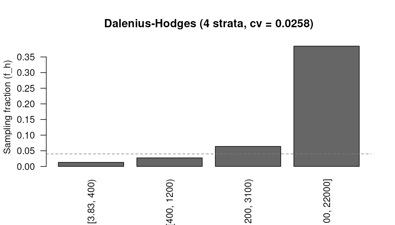

Visualizing allocation

plot() shows the sampling fraction per stratum. Under Neyman allocation, high-variance strata are sampled more intensively. The dashed line marks the overall fraction:

plot(sb)

Handing boundaries to the allocator

$strata carries the N, sd, and mean columns n_alloc() needs, so the two halves of a stratified design connect directly:

sb_cv <- strata_bound(x, n_strata = 4, cv = 0.05, method = "lh")
n_alloc(sb_cv$strata, cv = 0.05)
#> Stratum allocation (neyman, 4 strata)
#> field design: n = 59, cv = 0.0490, cost = 59
#> continuous optimum: n = 56.83406, cv = 0.0500, se = 40.3814
#> (deff = 1)
#> design df = 55

Both functions evaluate the same variance, so cv means the same thing to each and n is a fielded sample in both. Design assumptions carry across unchanged, whether passed directly or through a svyplan() profile:

plan <- svyplan(deff = 1.8, resp_rate = 0.85)
sb_deff <- strata_bound(x, n_strata = 4, cv = 0.05, plan = plan)
sb_deff$n
#> [1] 118
n_alloc(sb_deff$strata, cv = 0.05, plan = plan)$n
#> [1] 116.4128

The remaining gap between the two totals is integer rounding, not a difference in model: strata_bound() reports the whole-unit allocation in $strata$n, while n_alloc() reports the continuous optimum.

A scalar deff does not move the cut points. It scales the variance of every candidate boundary set equally, so what it changes is the n a target requires, not where the strata divide.

Stratified allocation

Given a sampling frame with stratum population sizes (N) and stratum standard deviations (sd), n_alloc() distributes a total sample across strata. This is the second half of a stratified design: strata_bound() finds the cut points, and n_alloc() allocates within strata.

frame <- data.frame(
  N = c(4000, 3000, 3000),
  sd = c(10, 15, 8),
  mean = c(50, 60, 55)
)

# Fixed total n with Neyman allocation
n_alloc(frame, n = 600, alloc = "neyman")
#> Stratum allocation (neyman, 3 strata)
#> field design: n = 600, cv = 0.0079, cost = 600
#> continuous optimum: n = 600, cv = 0.0079, se = 0.4305
#> (deff = 1)
#> design df = 597

Three solve modes are available: fixed total n, target cv, or budget constraint (when unit_cost is provided in the frame).

Constraints and domain-level targets are often the more practical use cases:

frame_constraints <- transform(
  frame,
  unit_cost = c(1, 1.5, 1),
  max_weight = c(25, 20, NA),
  take_all = c(FALSE, FALSE, TRUE)
)

n_alloc(frame_constraints, budget = 3500, alloc = "optimal", min_n_stratum = 40)
#> Stratum allocation (optimal, 3 strata)
#> field design: n = 3403, cv = 0.0076, cost = 3500
#> continuous optimum: n = 3403.425, cv = 0.0076, se = 0.4125
#> (min_n_stratum = 40, deff = 1)
#> design df = 401

frame_domains <- data.frame(
  province = c("North", "North", "South", "South"),
  stratum = c("Urban", "Rural", "Urban", "Rural"),
  N = c(2000, 3000, 1800, 3200),
  sd = c(12, 18, 10, 16),
  mean = c(55, 48, 58, 50)
)

# Minimum total n such that each province meets the CV target
n_alloc(frame_domains, domains = "province",
        cv = 0.04, alloc = "power", alloc_q = 0.3)
#> Stratum allocation (power, 4 strata)
#> field design: n = 112, cv = 0.0270, cost = 112
#> continuous optimum: n = 110.7422, cv = 0.0272, se = 1.4076
#> (deff = 1)
#> design df = 108
#> Domains: 2
#> 
#>  province .domain .n       .se      .moe     .rmoe      .cv    .cost
#>  North    5_North 59.23404 2.032000 3.982647 0.07839856 0.0400 59   
#>  South    5_South 51.50815 1.948447 3.818886 0.07221797 0.0368 52

prec_alloc() computes the achieved precision for any allocation:

prec_alloc(frame, n = c(200, 250, 150))
#> Sampling precision for alloc
#> n = 600 (3 strata)
#> se = 0.4321, moe = 0.8469, cv = 0.0079, rmoe = 0.0155

$detail carries the same numbers per stratum, so you can see where the precision is actually being bought. .share is the stratum’s contribution to the design variance of the overall mean and sums to 1:

prec_alloc(frame, n = c(200, 250, 150))$detail[, c("stratum", "n", ".se", ".cv", ".share")]
#>   stratum   n       .se        .cv    .share
#> 1       1 200 0.6892024 0.01378405 0.4070048
#> 2       2 250 0.9082951 0.01513825 0.3976329
#> 3       3 150 0.6366579 0.01157560 0.1953623

With domains, $domains reports the same table n_alloc() returns, so a design and its assessment compare row for row.

Fieldwork that differs across strata

deff and resp_rate take one value per stratum, either as vectors or as frame columns, for designs whose fieldwork is not uniform. A response rate that varies changes where the sample should go, not just how much of it comes back:

uneven <- data.frame(
  stratum   = c("Urban", "Peri-urban", "Rural"),
  N         = c(4000, 3000, 3000),
  sd        = c(10, 15, 8),
  mean      = c(50, 60, 55),
  resp_rate = c(0.92, 0.80, 0.65)
)
n_alloc(uneven, n = 600, alloc = "neyman")$detail[, c("stratum", "n", "n_int")]
#>      stratum        n n_int
#> 1      Urban 205.4620   205
#> 2 Peri-urban 247.8752   248
#> 3      Rural 146.6628   147

A value shared by every stratum is a constant factor that cancels out of a proportional weighting, so scalar deff and resp_rate behave exactly as before.

Joint indicator and domain targets

When one allocation must satisfy several estimands, use an atomic frame plus long measures and targets tables. Atomic means that every frame row has a single value for every domain classification in use. The example below crosses region and residence, allowing those two domain systems to overlap without requiring separate public functions or an alloc selector.

joint_frame <- data.frame(
  stratum = c("NU", "NR", "SU", "SR"),
  region = c("North", "North", "South", "South"),
  residence = c("Urban", "Rural", "Urban", "Rural"),
  N = c(1000, 2000, 1500, 1000),
  unit_cost = c(1, 1.2, 1.5, 1)
)

joint_measures <- data.frame(
  stratum = rep(joint_frame$stratum, 2),
  name = rep(c("vaccination", "income"), each = 4),
  p = c(0.50, 0.40, 0.60, 0.30, rep(NA, 4)),
  mean = c(rep(NA, 4), 50, 55, 60, 45),
  sd = c(rep(NA, 4), 10, 12, 15, 9)
)

joint_targets <- data.frame(
  name = c("vaccination", "vaccination", "income"),
  domain = c(".overall", "region", "residence"),
  level = c(NA, "North", "Urban"),
  cv = c(0.05, 0.08, NA),
  moe = c(NA, NA, 2)
)

joint_fit <- n_alloc(
  joint_frame,
  measures = joint_measures,
  targets = joint_targets,
  min_n_stratum = 2
)
joint_fit
#> Joint constrained allocation (Bethel)
#> question: cheapest design meeting every precision target
#> field design: n = 425, cost = 508 (3 targets, all pass)
#> continuous optimum: n = 424.8282, cost = 508 (integerizing costs +0.04%)
#> binding: vaccination@.overall:cv (target 0.05, achieved 0.05)
joint_fit$constraints
#>                    constraint        name    domain level .metric .target
#> 1     vaccination@.overall:cv vaccination  .overall  <NA>      cv    0.05
#> 2 vaccination@region=North:cv vaccination    region North      cv    0.08
#> 3  income@residence=Urban:moe      income residence Urban     moe    2.00
#>    .achieved    .ratio     .residual .tolerance        .se        .cv
#> 1 0.05000000 1.0000000  1.782579e-10      1e-06 0.02272727 0.05000000
#> 2 0.07030489 0.8788112 -1.211888e-01      1e-06 0.03046545 0.07030489
#> 3 1.85333281 0.9266664 -7.333360e-02      1e-06 0.94559534 0.01688563
#>         .moe      .rmoe .pass .binding .multiplier .sensitivity
#> 1 0.04454464 0.09799820  TRUE     TRUE  0.03000152    -18750.95
#> 2 0.05971119 0.13779506  TRUE    FALSE  0.00000000         0.00
#> 3 1.85333281 0.03309523  TRUE    FALSE  0.00000000         0.00

The optimizer minimizes variable cost subject to all three requirements. joint_fit$detail$n is the continuous optimum and joint_fit$detail$n_int is the deterministic feasible operational recommendation. The latter is locally cleaned but is not claimed to be a globally optimal integer solution. Both precision tables are retained:

prec_alloc(joint_fit)
#> Joint allocation precision (3 constraints)
#> targets: all pass
#> showing 1 binding of 3
#> 
#>  constraint              .metric .target .achieved .pass
#>  vaccination@.overall:cv cv      0.05    0.05      TRUE 
#> 
#> ... see $detail for all rows
prec_alloc(joint_fit, n = joint_fit$detail$n_int)
#> Joint allocation precision (3 constraints)
#> targets: all pass

A modified named allocation can be assessed in any order because names are matched exactly to frame$stratum.

Fixed-take multistage joint allocation

The same public interface supports two- and three-stage designs when every later-stage take is fixed. The frame owns stage populations, takes, and costs; the measures table owns indicator-specific stage homogeneity parameters. Only n_psu is optimized. Public n, planning bounds, and precision assessments remain in ultimate-unit units.

This three-stage example samples PSUs, then a fixed number of SSUs per PSU, then a fixed number of ultimate units per SSU:

joint_frame_3stage <- within(joint_frame, {
  unit_cost <- NULL
  N_psu <- c(100, 160, 120, 90)
  N_ssu <- c(600, 1200, 900, 500)
  n_per_psu <- c(8, 10, 12, 7)
  n_per_ssu <- c(4, 5, 3, 4)
  cost_psu <- c(300, 400, 450, 350)
  cost_ssu <- c(25, 30, 35, 28)
  cost_tsu <- c(5, 6, 7, 5)
})

joint_measures_3stage <- transform(
  joint_measures,
  icc_psu = rep(c(0.03, 0.05, 0.08, 0.04), 2),
  icc_ssu = rep(c(0.10, 0.08, 0.12, 0.06), 2),
  var_ratio_psu = 1,
  var_ratio_ssu = 1
)

joint_fit_3stage <- n_alloc(
  joint_frame_3stage,
  measures = joint_measures_3stage,
  targets = joint_targets,
  min_n_stratum = 20
)
joint_fit_3stage$detail[, c(
  "stratum", "n_psu_int", "n_per_psu", "n_per_ssu", "n_int"
)]
#>   stratum n_psu_int n_per_psu n_per_ssu n_int
#> 1      NU         6         8         4   192
#> 2      NR        11        10         5   550
#> 3      SU         9        12         3   324
#> 4      SR         5         7         4   140
prec_alloc(joint_fit_3stage, n = joint_fit_3stage$detail$n_int)
#> Joint allocation precision (3 constraints)
#> targets: all pass

The exact operational identity is n_int = n_psu_int * n_per_psu * n_per_ssu. N_psu is required for both multistage forms, while three-stage frames also require the stratum’s total N_ssu. Fixed takes must be whole numbers. take_all is unavailable because taking every PSU alone does not establish a census of ultimate units.

Stratified two-stage designs

Most household surveys stratify first and cluster within each stratum, sampling enumeration areas and then households. Adding a icc_psu column to the frame switches n_alloc() to this design. The per-stratum homogeneity can come straight from varcomp() with strata, whose output columns are named to match the frame:

set.seed(3)
listing <- data.frame(
  region = rep(c("North", "South"), each = 600),
  ea = rep(1:60, each = 20),
  income = rnorm(1200, rep(c(50, 70), each = 600), 15) +
    rep(rnorm(60, 0, 6), each = 20)
)
vc_region <- varcomp(income ~ ea, data = listing, strata = ~region)
vc_region
#> Variance components (2-stage, 2 strata)
#> 
#>  stratum sd      mean    icc_psu var_ratio_psu varb   varw   unit_relvar
#>  North   15.6736 51.1316 0.1056  1.0489        0.0104 0.0882 0.0940     
#>  South   16.0116 69.3691 0.1595  1.0479        0.0089 0.0469 0.0533

frame_2stage <- merge(
  data.frame(stratum = c("North", "South"), N = c(40000, 60000)),
  as.data.frame(vc_region)[, c("stratum", "sd", "mean", "icc_psu", "var_ratio_psu")],
  by = "stratum"
)
frame_2stage$cost_psu <- c(400, 550)
frame_2stage$cost_ssu <- c(45, 60)

res_2stage <- n_alloc(frame_2stage, cv = 0.02)
res_2stage
#> Stratum allocation (neyman, two-stage, 2 strata)
#> field design: n = 338, n_psu = 44, cv = 0.0197, cost = 40205
#> continuous optimum: n = 323.6245, cv = 0.0200, se = 1.2415
#> (deff = 1)
#> design df = 42
res_2stage$detail[, c("stratum", "n_int", "n_per_psu", "n_psu_int")]
#>   stratum n_int n_per_psu n_psu_int
#> 1   North   135  8.675795        15
#> 2   South   203  6.951041        29

Each stratum gets its cost-optimal cluster take (fix it instead with a n_per_psu column), and the PSU counts fall out of the element allocation. Budget mode, min_n_stratum, and max_weight work the same way here. take_all does not apply: taking every PSU leaves the within-PSU take in force, so it does not enumerate a stratum, and it is refused rather than half-honoured.

An N_psu column caps each stratum at the PSUs it actually has, both in the continuous allocation and in the whole-unit design. Without it the allocation can ask for more clusters than a stratum contains:

frame_bounded <- frame_2stage
frame_bounded$N_psu <- c(40, 900)

res_bounded <- n_alloc(frame_bounded, n = 3000)
res_bounded$detail[, c("stratum", "n_psu", "n_psu_int", "N_psu",
                       ".psu_frac", ".bound_source")]
#>   stratum    n_psu n_psu_int N_psu .psu_frac .bound_source
#> 1   North  40.0000        40    40 1.0000000         N_psu
#> 2   South 381.6649       379   900 0.4240721          <NA>

North holds only 40 enumeration areas, so its allocation stops there and .bound_source names the constraint that stopped it. Asking for precision the remaining PSUs cannot deliver is an error rather than a silent overshoot, and it says the ceiling came from PSU availability under a with-replacement first stage rather than from the population.

N_psu is a feasibility constraint only. It does not switch on a first-stage finite population correction, so precision still uses a with-replacement first stage and stays conservative when a design takes an appreciable share of the available PSUs. print() says so when that happens, and .psu_frac reports the share.

Two-phase designs

In a two-phase (or double) sample, a large cheap phase 1 measures something that helps target the expensive measurement, and a subsample is carried into phase 2. n_twophase() allocates both phases at once, minimizing cost for a target CV or CV for a fixed budget.

The frame is one row per phase-2 stratum, similarly to what is used in n_alloc() :

frame <- data.frame(
  stratum   = c("A", "B", "C", "D"),
  N         = c(3500, 2500, 2500, 1500),
  sd        = c(12, 25, 8, 40),
  mean      = c(40, 70, 35, 90),
  unit_cost = c(2, 5, 1, 9)
)

n_twophase(frame, phase1_cost = 1, budget = 50000)
#> Two-phase allocation (4 phase-2 strata)
#> field design: n_phase1 = 16924 | n_phase2 = 8094
#> cv = 0.0050, cost = 50000
#> 
#>  stratum share    sd unit_cost     nu n_int
#>        A 0.350 12.00      2.00 0.4154  2462
#>        B 0.250 25.00      5.00 0.5474  2316
#>        C 0.250  8.00      1.00 0.3917  1659
#>        D 0.150 40.00      9.00 0.6528  1657
#> 
#> single-phase is better here: n = 14085 at cv 0.0046, so skip phase 1
#> # summary() for the continuous optimum and the comparator

The nu column is the fraction of each phase-1 stratum carried forward. Its shape is Neyman-like, proportional to $S_h/\sqrt{c_h}$, but the overall scale is set by the between-stratum variance: the weaker the stratification, the closer every fraction moves to 1, meaning keep everything phase 1 found.

Two design effects, not one

Neither phase has to be a simple random sample, and the two carry separate design effects because they apply to different things. phase1_deff inflates the between-stratum component, the part phase 1 is responsible for. A deff column inflates each stratum’s within-stratum residual, the part phase 2 has to measure. single_deff describes the comparator, which need not be fielded like phase 2.

clustered <- transform(frame, deff = c(1.2, 2.5, 0.8, 1.7))

n_twophase(clustered, phase1_cost = 1, budget = 50000,
           phase1_deff = 2.2, single_deff = 2.9)
#> Two-phase allocation (4 phase-2 strata)
#> field design: n_phase1 = 17999 | n_phase2 = 7172
#> cv = 0.0070, cost = 50000
#> phase-1 deff = 2.20, single-phase deff = 2.90
#> 
#>  stratum share    sd unit_cost deff     nu n_int
#>        A 0.350 12.00      2.00 1.20 0.3068  1933
#>        B 0.250 25.00      5.00 2.50 0.5835  2626
#>        C 0.250  8.00      1.00 0.80 0.2362  1064
#>        D 0.150 40.00      9.00 1.70 0.5738  1549
#> 
#> single-phase alternative: n = 14085 at cv 0.0079, two-phase wins
#> # summary() for the continuous optimum and the comparator

Inflating the combined variance by one design effect instead would be a different and wrong model. The two also pull against each other, and the trap runs in the direction that looks attractive: a stratifier built purely from between-cluster structure shrinks the residual, lowering the stratum deff, but it makes the fitted values nearly constant within clusters and so drives phase1_deff up toward the cluster size. Under a clustered phase 1 that first term can dominate, and the design loses to a plain sample even though the residual design effect looks favorable.

Every result carries the single-phase comparison, because two-phase sampling is not always an improvement. Skipping phase 1 and measuring directly can be both cheaper and more precise when the screener costs too much or the stratifier predicts too little, and the print output says so when that happens.

Response rates

Both phases can lose sample to nonresponse, and the two enter separately. resp_rate is the phase-1 response or successful-classification rate; a resp_rate column is the phase-2 completion rate in each stratum. Response divides its own component, exactly as the design effects do, so a stratum that responds poorly is subsampled differently rather than the whole design being inflated by one factor.

screened <- transform(frame, resp_rate = c(0.9, 0.7, 0.85, 0.6))

n_twophase(screened, phase1_cost = 1, budget = 50000, resp_rate = 0.8)
#> Two-phase allocation (4 phase-2 strata)
#> field design: n_phase1 = 16034 | n_phase2 = 7880
#> expected responding: n_phase1 = 12827 | n_phase2 = 6003
#> cv = 0.0059, cost = 50000
#> 
#>  stratum share    sd unit_cost resp     nu n_int n_resp
#>        A 0.350 12.00      2.00 0.90 0.3917  2198   1978
#>        B 0.250 25.00      5.00 0.70 0.5852  2346   1642
#>        C 0.250  8.00      1.00 0.85 0.3800  1523   1295
#>        D 0.150 40.00      9.00 0.60 0.7538  1813   1088
#> 
#> single-phase is better here: n = 14085 at cv 0.0046, so skip phase 1
#> # summary() for the continuous optimum and the comparator

Everything here counts units issued, so a cost quoted per completed interview has to be converted first: c_contact + resp_rate * c_complete. Issued and expected-responding counts are reported separately, because they are different quantities and neither is an effective sample size. There is no single effective size for a two-phase design, since the two variance components carry different design effects.

Phase 2 can only draw from what phase 1 managed to classify, so every subsampling fraction is capped at the phase-1 response rate.

One caveat worth stating plainly: dividing by a response rate assumes response is ignorable within the strata you supplied. That is a substantive claim about the strata, not a property of the arithmetic, and no sample size removes nonresponse bias. Where the assumption is uncomfortable, modeling the nonresponse as a follow-up phase is the alternative the design itself offers.

When the phase-1 sample is already fixed

Often it is. The screener has run, or phase 1 is an existing survey, a panel, or a listing operation sized by field capacity rather than by this design. Phone surveys built on a previous face-to-face round are the common case. Supply n_phase1 and the only decision left is how deep to subsample.

n_twophase(frame, phase1_cost = 1, budget = 50000, n_phase1 = 20000)
#> Two-phase allocation (4 phase-2 strata)
#> field design: n_phase1 = 20000 | n_phase2 = 7340
#> cv = 0.0051, cost = 50000
#> 
#>  stratum share    sd unit_cost     nu n_int
#>        A 0.350 12.00      2.00 0.3189  2232
#>        B 0.250 25.00      5.00 0.4202  2101
#>        C 0.250  8.00      1.00 0.3006  1504
#>        D 0.150 40.00      9.00 0.5011  1503
#> 
#> single-phase is better here: n = 14085 at cv 0.0046, so skip phase 1
#> # summary() for the continuous optimum and the comparator

The relative allocation is unchanged, because it is $S_h\sqrt{d_{2h}/c_h}$ in every mode. What moves is the overall scale, now pinned by the budget left after paying for phase 1 rather than by the variance-cost trade-off. Since the optimizing choice of n_phase1 is the best member of this family, fixing it can only match or lose to leaving it free, and the difference is what a phase-1 size you did not choose is costing you.

Two things can go wrong, and both give a specific error. The budget may not reach phase 2 at all. Or a target CV may sit below the phase-1 variance floor: what that n_phase1 leaves when every classified unit is carried into phase 2, which is

$$\frac{1}{\mu}\sqrt{\frac{1}{n_a}\left(\frac{d_1A}{r_1} + \sum_h \frac{d_{2h}W_hS_h^2}{r_{2h}r_1}\right) - \frac{d_1A + \sum_h d_{2h}W_hS_h^2}{N}}.$$

The between-stratum term is the part already paid for by the phase-1 size. It is not the whole floor, though, because subsampling stops at the classification rate rather than at 1, so the phase-2 residual survives at $\nu_h = r_1$ and is added to it. The subtracted term is the finite population correction, and it is what makes the floor vanish at a census: with $n_a = N$ and no losses the two halves cancel exactly. It carries the design effects, since those inflate an SRSWOR variance here as everywhere, but not the response rates, because measuring every unit removes all the variance while failing to reach some of them does not.

Whole units and assurance

$operational carries the field design in whole units, and it is what the printed block reports: every count there is a whole unit off the same solution, so the phase sizes, the stratum takes and the responding figures reconcile. Budget mode floors and then buys back units in order of variance reduction per unit cost, staying inside the budget; CV mode rounds up, overshooting precision rather than missing it. summary() sets the continuous optimum beside the fielded design and gives the single-phase comparator in full.

Planning at the expected respondent count leaves roughly half of all designs short. assurance reports the issue for which the required respondents arrive with at least that probability, from the binomial distribution of respondents:

screened <- transform(frame, resp_rate = c(0.9, 0.7, 0.85, 0.6))

n_twophase(screened, phase1_cost = 1, budget = 50000,
           resp_rate = 0.8, assurance = 0.90)
#> Two-phase allocation (4 phase-2 strata)
#> field design: n_phase1 = 16034 | n_phase2 = 7880
#> expected responding: n_phase1 = 12827 | n_phase2 = 6003
#> cv = 0.0059, cost = 50000
#> 
#>  stratum share    sd unit_cost resp     nu n_int n_resp
#>        A 0.350 12.00      2.00 0.90 0.3917  2198   1978
#>        B 0.250 25.00      5.00 0.70 0.5852  2346   1642
#>        C 0.250  8.00      1.00 0.85 0.3800  1523   1295
#>        D 0.150 40.00      9.00 0.60 0.7538  1813   1088
#> 
#> assured (0.90): issue n_phase1 = 16116 | n_phase2 = 8010 (cost 50761)
#> single-phase is better here: n = 14085 at cv 0.0046, so skip phase 1
#> # summary() for the continuous optimum and the comparator

If the assured phase-2 issue exceeds the pool phase 1 supplies, that is a signal to enlarge phase 1 rather than to over-issue.

Nonresponse follow-up

Following up a subsample of nonrespondents is the same allocation problem with two strata. The respondents are already measured, so they cost nothing more and are all kept, which is unit_cost = 0 with take_all = TRUE. Only the nonrespondents are subsampled:

theta <- 0.5   # phase-1 response rate

nrfu <- data.frame(
  stratum   = c("respondents", "nonrespondents"),
  N         = c(theta, 1 - theta),
  sd        = c(1, 1),
  unit_cost = c(0, 200),
  take_all  = c(TRUE, FALSE)
)

n_twophase(nrfu, phase1_cost = 50, budget = 100000,
           mu = 1, single_cost = 50 / theta)
#> Two-phase allocation (2 phase-2 strata)
#> field design: n_phase1 = 828 | n_phase2 = 707
#> cv = 0.0382, cost = 1e+05
#> 
#>         stratum share   sd unit_cost     nu n_int take_all
#>     respondents 0.500 1.00      0.00 1.0000   414        *
#>  nonrespondents 0.500 1.00    200.00 0.7071   293         
#> 
#> single-phase is better here: n = 1000 at cv 0.0316, so skip phase 1
#> # summary() for the continuous optimum and the comparator

The optimal follow-up fraction reduces to $\sqrt{c_1/(c_2\theta)}$ here, the standard result. Two details matter in this configuration. single_cost: a unit_cost of 0 means “already measured”, not “free”, so the baseline for the comparison has to be named explicitly as the cost of one completed interview without follow-up. And resp_rate should stay at its default of 1, because here the strata are response status, so classification succeeds for every unit and setting a phase-1 rate as well would count the same loss twice.

Change and panel designs

The families above size one occasion. A survey that runs more than once is sized against a different quantity: the change between two occasions, and, if the same units are followed, how many to recruit so that enough of them are still responding later.

Sizing a change

n_change() and prec_change() are the n_*/prec_* pair for a change in a mean or a proportion. Two independent rounds cost twice a single occasion:

n_change(p = c(0.30, 0.36), moe = 0.02)
#> Sample size for change (proportion scale)
#> n = 4230 per occasion (p = 0.3 to 0.36, moe = 0.02, deff = 1)
#> No between-occasion covariance (overlap x overlap_cor = 0)

Measuring the same units twice is cheaper, because the change is a difference and the unit-level correlation cancels part of it. Two arguments describe that, and only their product buys anything: overlap is the share of the first occasion’s responding sample measured again, and overlap_cor the correlation among those shared units. A full panel of uncorrelated measurements saves nothing.

n_change(p = c(0.30, 0.36), moe = 0.02, overlap = 0.75, overlap_cor = 0.5)
#> Sample size for change (proportion scale)
#> n = 2646 per occasion (p = 0.3 to 0.36, moe = 0.02, deff = 1)
#> overlap = 0.75, overlap_cor = 0.5 (62.5% of the independent variance)

The pair round-trips like every other:

res <- n_change(p = c(0.30, 0.36), moe = 0.02, overlap = 0.75, overlap_cor = 0.5)
prec_change(res)$moe
#> [1] 0.02

overlap and overlap_cor come from different places, and it is worth keeping them apart. The overlap is a property of the design and is fixed once the rotation is declared. The correlation is a property of the variable and has to come from a previous round of the same survey.

Overlap from a rotation schedule

design_overlap() supplies the design half. Give it the occasions a unit spends in and out of sample over its whole life, as a compact spec naming the spells in order from in sample, and it returns the overlap at every lag the schedule reaches:

cps <- design_overlap("4-8-4")
cps[c(1, 12)]
#> [1] 0.75 0.50

Those are the two published CPS figures: 75 percent of the sample is shared between consecutive months, 50 percent between the same month a year apart. A schedule is a finite life, not a repeating pattern, and the difference is invisible in the answer. Read "4-8-4" as “four in, eight out, repeat” and only the group finishing its stint leaves each month, which gives 87.5 percent. The finite life loses a group at the end of each of its two spells, keeps six of eight, and gives the published 75 percent. A compact spec with an even number of spells could only mean a cycle and is refused.

Each lag is a different design question, so name the one the change spans rather than passing the profile whole:

c(consecutive = n_change(p = c(0.30, 0.36), moe = 0.02,
                         overlap = cps[1], overlap_cor = 0.5)$n,
  annual = n_change(p = c(0.30, 0.36), moe = 0.02,
                    overlap = cps[12], overlap_cor = 0.5)$n)
#> consecutive      annual 
#>    2645.106    3173.220

Two notations for a schedule are in print, and both are accepted. "4-8-4" counts occasions per spell, which is how the CPS pattern is written. "1-1-0-0-1-1" carries one flag per occasion, which is how Lynn (2012) writes the same kind of design. They are told apart by the 0, which no spell can be. A string of all 1s is a valid sentence in both and a different design in each, so it is refused rather than resolved by precedence. "1-1-1" is three consecutive occasions as a pattern and one in, one out, one in as spells. Their consecutive overlaps are 2/3 and 0. Write "3" or "1-0-1".

plot() draws the schedule as the chart these designs are published as, one row per cohort and one column per time period:

plot(design_overlap("1-1-0-0-1-1"))

A cohort enters at every period drawn, so the total row climbs through the launch and settles at the sample the overlaps divide by, which is marked. Everything left of that mark is the gradual start a rotating design has: reaching the intended sample takes a full life unless the first period’s sample is deliberately split into cohorts of unequal life, which one schedule does not express.

One conversion is the planner’s to make. design_overlap() counts the units the design issues at both occasions, while overlap in the sizing and power functions is the share of the first occasion’s respondents measured again. The two are the same number at full response. Below it they are not, and converting between them needs an assumption about how response persists across occasions, which the package does not make: under response independent between occasions at rate r, an issued overlap f leaves about f * r among respondents, rising towards f as respondents become likelier to respond again.

Recruiting a panel that loses units

A panel loses units at every wave, so the sample that carries the analysis is smaller than the one recruited. n_panel() sizes the recruitment. It does not restate the arguments of n_prop() or n_mean(). It takes one of their results and reads it as both the responding sample to reach and the estimand to report precision for.

The rates below are the UK LFS: 73 percent response at recruitment, then quarterly retention of a surviving cohort.

target <- n_prop(p = 0.5, moe = 0.031)
lfs <- n_panel(target, retention = c(0.878, 0.963, 0.936, 0.956),
               resp_rate = 0.728)
lfs
#> Panel recruitment (fixed, 5-wave life)
#> issued: 1815 -> 1000 responding at wave 5
#> proportion (wald): se = 0.01582, moe = 0.031, cv = 0.0316
#> 
#>  wave retention n_resp se      moe    
#>  1              1321   0.01376 0.02696
#>  2    0.878     1160   0.01468 0.02878
#>  3    0.963     1117   0.01496 0.02932
#>  4    0.936     1046   0.01546 0.03031
#>  5    0.956     1000   0.01582 0.031  
#> 
#> # summary() for the launch, the loss and per-wave cv

The printed block is the answer: what to issue, what it leaves, and the precision at each wave. summary() gives what the answer rests on, including the rates assumed, where the life’s loss falls, the cv and expected cases at each wave, and for a rotating design the standing sample and the launch.

resp_rate and retention are separate arguments because a panel’s loss is concentrated at recruitment. Here 61 percent of the whole five-wave loss happens at wave 1, and an average rate spread over the waves would under-issue.

lfs$waves[, c("wave", "q", "loss_share", "n_resp", "moe")]
#>   wave         q loss_share    n_resp        moe
#> 1    1 0.7280000 0.60550724 1320.8645 0.02696429
#> 2    2 0.6391840 0.19771592 1159.7190 0.02877675
#> 3    3 0.6155342 0.05264754 1116.8094 0.02932436
#> 4    4 0.5761400 0.08769657 1045.3336 0.03031033
#> 5    5 0.5507898 0.05643274  999.3389 0.03100000

target_wave sizes for a precision reached earlier than the last wave, with the later waves still reported.

The same rates can be run as a rotating panel, where an equal cohort enters every occasion and the estimate pools every cohort alive. That returns a different quantity, so it has a different name:

rot <- n_panel(target, retention = c(0.878, 0.963, 0.936, 0.956),
               resp_rate = 0.728, design = "rotating")
c(entrants = rot$n_entrants, in_sample = rot$n_in_sample)
#>  entrants in_sample 
#>  321.3672 1606.8361

n_entrants is what the design takes on each occasion once it is running. n_in_sample is what its five live cohorts hold between them, which is also the cumulative recruitment that reaching a steady state takes. On these rates they differ by a factor of five, and reading one as the other is the mistake the two names exist to prevent.

Every figure so far is an expected value, which leaves about half of all panels short of the target. assurance reports the recruitment that clears it with a stated probability instead:

n_panel(target, retention = c(0.878, 0.963, 0.936, 0.956),
        resp_rate = 0.728, assurance = 0.90)$n_assured
#> [1] 1865

For a fixed panel that inverts one binomial tail. For a rotating one the respondents at an occasion are a sum of binomials at different cumulative probabilities, one per live cohort, which is a Poisson-binomial and is computed exactly rather than approximated.

prec_panel() runs the pair in the other direction: given a recruitment already budgeted, it reports the responding sample and the precision left at each wave, and says so when that falls short of what the target needs.

Bringing a rotating design up

The recruitment above describes the design at a steady state, which it reaches once every stage of the life is represented at one occasion. How it gets there is a design decision. start = "gradual" recruits one cohort an occasion, so the sample climbs over a full life. start = "immediate" splits the first occasion into equal panels planned for life lengths from the full life down to one occasion. Every panel begins at its first interview, and together they hold the whole sample at once.

n_panel(target, retention = c(0.878, 0.963, 0.936, 0.956),
        resp_rate = 0.728, design = "rotating",
        start = "immediate")$launch[, c("period", "n_in_sample", "n_resp", "moe")]
#>   period n_in_sample    n_resp        moe
#> 1      1    1606.836 1169.7767 0.02865277
#> 2      2    1606.836 1055.6065 0.03016248
#> 3      3    1606.836 1032.8056 0.03049361
#> 4      4    1606.836 1007.4856 0.03087441
#> 5      5    1606.836  999.3389 0.03100000
#> 6      6    1606.836  999.3389 0.03100000

design_overlap() gives the same mature membership-overlap profile under either launch. A gradual launch has higher realized overlap while it fills because no full set of cohorts has yet rotated through. An immediate launch is in membership equilibrium at its first occasion and not in response equilibrium. Every unit there is at wave 1, so the occasion holds at least as many respondents as the design ever holds again, and strictly more as soon as any wave retains less than all of the one before. Here that is 1172 against the design’s 1001, temporarily more precise, converging down as the interview mix matures. The two coincide only where nothing is lost after recruitment. A gradual launch approaches the same respondent figure from below, at 234. $launch_waves decomposes each occasion into the interviews represented in the sample, which is where both launch paths show.

Either way the early occasions rest on a different response composition from the rest of the series, and that, rather than the sample size, is what makes them hard to compare with it.

design_schedule() turns that launch into an operational manifest without drawing a sample. The horizon policy is explicit: "continuing" records interviews owed after the reporting window, "truncate_lives" ends those lives at the window, and "close_intake" stops recruiting early enough for every cohort to finish. Rounding is explicit too and is applied to each panel before startup panels are summed.

rot_launch <- n_panel(
  target,
  retention = c(0.878, 0.963, 0.936, 0.956),
  resp_rate = 0.728,
  design = "rotating",
  start = "immediate"
)
field_plan <- design_schedule(
  rot_launch,
  life = design_overlap("5"),
  horizon = 8,
  horizon_policy = "continuing",
  refreshment = "entrant_register",
  rounding = "ceiling"
)
field_plan
#> Longitudinal design schedule (immediate launch, continuing)
#> life: 5 stages over 8 occasions, steady from occasion 5
#> rounding: ceiling at panel and cohort level
#> issue: 1610 at startup, 322 per occasion (occasions 2-8)
#> tail commitments: 10 panel-interviews after occasion 8
#> # summary() for the occasion-by-occasion profile and the overlap
field_plan$components[, c("cohort", "entry_wave", "operational_issue",
                          "panels", "frame_role")]
#>     cohort entry_wave operational_issue panels       frame_role
#> 1  startup          1              1610      5          startup
#> 2 intake_2          2               322      1 entrant_register
#> 3 intake_3          3               322      1 entrant_register
#> 4 intake_4          4               322      1 entrant_register
#> 5 intake_5          5               322      1 entrant_register
#> 6 intake_6          6               322      1 entrant_register
#> 7 intake_7          7               322      1 entrant_register
#> 8 intake_8          8               322      1 entrant_register

A schedule’s length is set by the reporting horizon rather than by the design, so print() states the issue profile as the runs it is made of and stays the same size whether the window is six occasions or fifty-two. summary() gives the occasion-by-occasion tables. The dense $schedule table marks every component-panel combination active or inactive at each in-horizon occasion. $tail_commitments contains only the promised interviews after the horizon. An entrant register means the later frames contain new eligible units. If later cohorts instead use whole frame vintages, declare refreshment = "whole_vintage" and construct their combined analysis weights outside this planning object.

plot(design_overlap("5"), start = "immediate")

Averaging occasions, and the trade-off that makes

A repeated survey rarely publishes only single occasions and changes between them. An annual average built from quarterly rounds is an estimate in its own right, and it is the one place a rotation costs rather than pays. prec_pooled() and n_pooled() size it, on the equal-weight mean of the occasion estimates.

prec_pooled(var = 100, n = 500, occasions = 4)
#> Sampling precision for pooled estimate (mean scale)
#> n = 500 per occasion, 4 occasions (var = 100, deff = 1)
#> No between-occasion covariance (overlap x overlap_cor = 0)
#> se = 0.2236, moe = 0.4383
prec_pooled(var = 100, n = 500, occasions = 4, overlap = 0.75, cor_decay = 0.8)
#> Sampling precision for pooled estimate (mean scale)
#> n = 500 per occasion, 4 occasions (var = 100, deff = 1)
#> overlap = 0.75, overlap_cor = 0.8 at lag 1, shared out to lag 3
#> se = 0.3586, moe = 0.7029

The second design shares three quarters of each round with the next and is markedly less precise on the annual figure. Overlap induces a positive covariance between occasions. That covariance is subtracted when you difference two occasions and added when you average them. It is positive whenever the overlap exceeds the sampling fraction n / N, which always holds here because there is no finite population correction. ?prec_pooled explains the boundary below it, where occasions share fewer units than chance and the two directions reverse. The correlation is stated per lag because a panel’s correlation falls away with distance. Here cor_decay = 0.8 gives the AR(1) shape, with correlation 0.8^m at lag m.

Three estimands and one design lever, priced together. The overlaps come from the schedule rather than being asserted:

horizon <- 8
arms <- function(life) {
  ov <- design_overlap(as.character(life), max_lag = horizon - 1)
  data.frame(
    span        = attr(ov, "life"),
    interviews  = sum(attr(ov, "schedule")),
    overlap_1   = round(as.numeric(ov)[1], 3),
    se_level    = round(prec_mean(var = 100, n = 1000, N = 1e5)$se, 4),
    se_change   = round(prec_change(var = 100, n = 1000, N = 1e5,
                                    overlap = ov[1], overlap_cor = 0.8)$se, 4),
    se_pooled   = round(prec_pooled(var = 100, n = 1000, N = 1e5,
                                    occasions = horizon, overlap = ov,
                                    cor_decay = 0.8)$se, 4)
  )
}
do.call(rbind, lapply(c(2, 4, 6, 8), arms))
#>   span interviews overlap_1 se_level se_change se_pooled
#> 1    2          2     0.500   0.3146    0.3458    0.1447
#> 2    4          4     0.750   0.3146    0.2821    0.1820
#> 3    6          6     0.833   0.3146    0.2574    0.2018
#> 4    8          8     0.875   0.3146    0.2441    0.2131

Reading down the columns: lengthening the life sharpens the change and blunts the annual average, while the single-occasion level does not move at all. The level is a function of that occasion’s size alone, so it is a horizontal reference line rather than a third position, and the trade-off is between the other two. A design serving both is sized by taking the larger of n_change() and n_pooled(), since neither dominates.

Two columns carry the burden because one cannot. span is the calendar distance from a unit’s first interview to its last and interviews is how many times it is actually asked. They coincide for an uninterrupted schedule and separate for a rotation with a rest period, where "4-8-4" spans sixteen occasions and asks eight.

gapped <- design_overlap("4-8-4")
c(span = attr(gapped, "life"), interviews = sum(attr(gapped, "schedule")))
#>       span interviews 
#>         16          8

The issued-versus-respondent conversion from earlier applies here too, and prec_pooled() enforces it rather than documenting it: a design_overlap() result is a statement about issued samples, so it is accepted directly at full response and refused below it, where the number you want is the respondent overlap you expect.

One refusal is worth recognising. A lag’s covariance changes sign once its overlap falls below the sampling fraction, and a covariance whose sign varies across lags need not be a covariance at all. prec_pooled() checks the assembled matrix, not the variance read off it, because a kernel that fails can still return a positive number:

prec_pooled(var = 100, n = 67000, occasions = 8, N = 1e5,
            overlap = design_overlap("4", max_lag = 7), cor_decay = 0.8)
#> Error:
#> ! the assembled between-occasion covariance is not a valid covariance (minimum eigenvalue -1.55e-05 against a diagonal of 0.000493); at a sampling fraction of 0.67 the covariance at lag 2 is negative, which happens once a lag's overlap falls below n/N. Over 8 occasions a rotation interviewing each cohort 4 times at this size draws 1.34 times the population, so the schedule could not be fielded either. Reduce the sampling fraction, shorten the horizon, or supply an overlap and correlation that hold together across lags

That is a municipality-scale sampling fraction, not an exotic corner, and the message names the fraction, the lag that turns, and whether the rotation would also exhaust its own population before the horizon is out.

Power analysis

Precision analysis answers “how precisely can we estimate a level?” Power analysis answers a different question: “can we detect a change or difference between two groups or time points?”

Sample size for a detectable change

A survey measured vaccination coverage at 70%. How many households are needed in a follow-up to detect a 5 percentage point increase with 80% power?

power_prop(p1 = 0.70, p2 = 0.75, power = 0.80)
#> Power analysis for proportions (solved for sample size)
#> n = 1248 (per group), power = 0.800, effect = 0.0500
#> (p1 = 0.700, p2 = 0.750, alpha = 0.05, deff = 1)

With a design effect:

power_prop(p1 = 0.70, p2 = 0.75, power = 0.80, deff = 2.0)
#> Power analysis for proportions (solved for sample size)
#> n = 2496 (per group), power = 0.800, effect = 0.0500
#> (p1 = 0.700, p2 = 0.750, alpha = 0.05, deff = 2.00)

Three solve modes

power_prop() and power_mean() each solve for whichever of n, power, or the effect size is left unspecified:

# Solve for n (default when p2 and power given)
power_prop(p1 = 0.70, p2 = 0.75, power = 0.80, deff = 2.0)
#> Power analysis for proportions (solved for sample size)
#> n = 2496 (per group), power = 0.800, effect = 0.0500
#> (p1 = 0.700, p2 = 0.750, alpha = 0.05, deff = 2.00)

# Solve for power (set power = NULL)
power_prop(p1 = 0.70, p2 = 0.75, n = 1500, power = NULL, deff = 2.0)
#> Power analysis for proportions (solved for power)
#> n = 1500 (per group), power = 0.584, effect = 0.0500
#> (p1 = 0.700, p2 = 0.750, alpha = 0.05, deff = 2.00)

# Solve for MDE (omit p2)
power_prop(p1 = 0.70, n = 1500, deff = 2.0)
#> Power analysis for proportions (solved for minimum detectable effect)
#> n = 1500 (per group), power = 0.800, effect = 0.0639
#> (p1 = 0.700, p2 = 0.764, alpha = 0.05, deff = 2.00)

Panel surveys

The power family takes the same overlap and overlap_cor as n_change(), and design_overlap() supplies the first of them from a rotation schedule. If the follow-up resamples a fraction of the original households and the between-round correlation is known, the required sample size drops:

power_prop(p1 = 0.70, p2 = 0.75, power = 0.80, deff = 2.0,
           overlap = 0.50, overlap_cor = 0.6)
#> Power analysis for proportions (solved for sample size)
#> n = 1749 (per group), power = 0.800, effect = 0.0500
#> (p1 = 0.700, p2 = 0.750, alpha = 0.05, deff = 2.00, overlap = 0.50, overlap_cor = 0.60)

Continuous outcomes

The same three solve modes work for means:

# Sample size to detect a difference of 5 (within-group var = 200)
power_mean(200, effect = 5)
#> Power analysis for means (solved for sample size)
#> n = 126 (per group), power = 0.800, effect = 5.0000
#> (alpha = 0.05, deff = 1)

# MDE with n = 400 per group
power_mean(200, n = 400)
#> Power analysis for means (solved for minimum detectable effect)
#> n = 400 (per group), power = 0.800, effect = 2.8016
#> (alpha = 0.05, deff = 1)

Difference-in-differences

power_did() handles two-group, two-period DiD designs. Specify treated and control group outcomes as c(baseline, endline) vectors:

# Proportion outcome: treated improves, control stable
power_did(treat = c(0.50, 0.55), control = c(0.50, 0.48),
          outcome = "prop", effect = 0.07)
#> Power analysis for DiD proportions (solved for sample size)
#> n = 1598 (per group), power = 0.800, effect = 0.0700
#> (treat = (0.500, 0.550), control = (0.500, 0.480), alpha = 0.05, deff = 1)

# Mean outcome with panel overlap
power_did(treat = c(50, 55), control = c(50, 52),
          outcome = "mean", var = 100, effect = 3,
          overlap = 0.5, overlap_cor = 0.6)
#> Power analysis for DiD means (solved for sample size)
#> n = 245 (per group), power = 0.800, effect = 3.0000
#> (treat = (50.000, 55.000), control = (50.000, 52.000), alpha = 0.05, deff = 1, var = (100.00, 100.00, 100.00, 100.00), overlap = 0.50, overlap_cor = 0.60)

Unequal groups and alternative methods

Both power_prop() and power_mean() support unequal group sizes via ratio or explicit n = c(n1, n2):

# 2:1 allocation ratio
power_prop(p1 = 0.30, p2 = 0.35, ratio = 2)
#> Power analysis for proportions (solved for sample size)
#> n1 = 2088, n2 = 1044 (total = 3132), power = 0.800, effect = 0.0500
#> (p1 = 0.300, p2 = 0.350, alpha = 0.05, deff = 1, ratio = 2)

# Unequal group variances
power_mean(c(80, 120), effect = 5)
#> Power analysis for means (solved for sample size)
#> n = 63 (per group), power = 0.800, effect = 5.0000
#> (alpha = 0.05, deff = 1)

For rare proportions, arcsine and log-odds transforms are more accurate:

power_prop(p1 = 0.15, p2 = 0.18, alternative = "one.sided",
           method = "arcsine")
#> Power analysis for proportions (solved for sample size)
#> n = 1890 (per group), power = 0.800, effect = 0.0300
#> (p1 = 0.150, p2 = 0.180, alpha = 0.05, deff = 1, one-sided, method = arcsine)

power_prop(p1 = 0.15, p2 = 0.18, alternative = "one.sided",
           method = "logodds")
#> Power analysis for proportions (solved for sample size)
#> n = 1889 (per group), power = 0.800, effect = 0.0300
#> (p1 = 0.150, p2 = 0.180, alpha = 0.05, deff = 1, one-sided, method = logodds)

Power curve

plot() draws the power-vs-sample-size curve with reference lines at the solved point:

pw <- power_prop(p1 = 0.70, p2 = 0.75, power = 0.80, deff = 2.0)
plot(pw)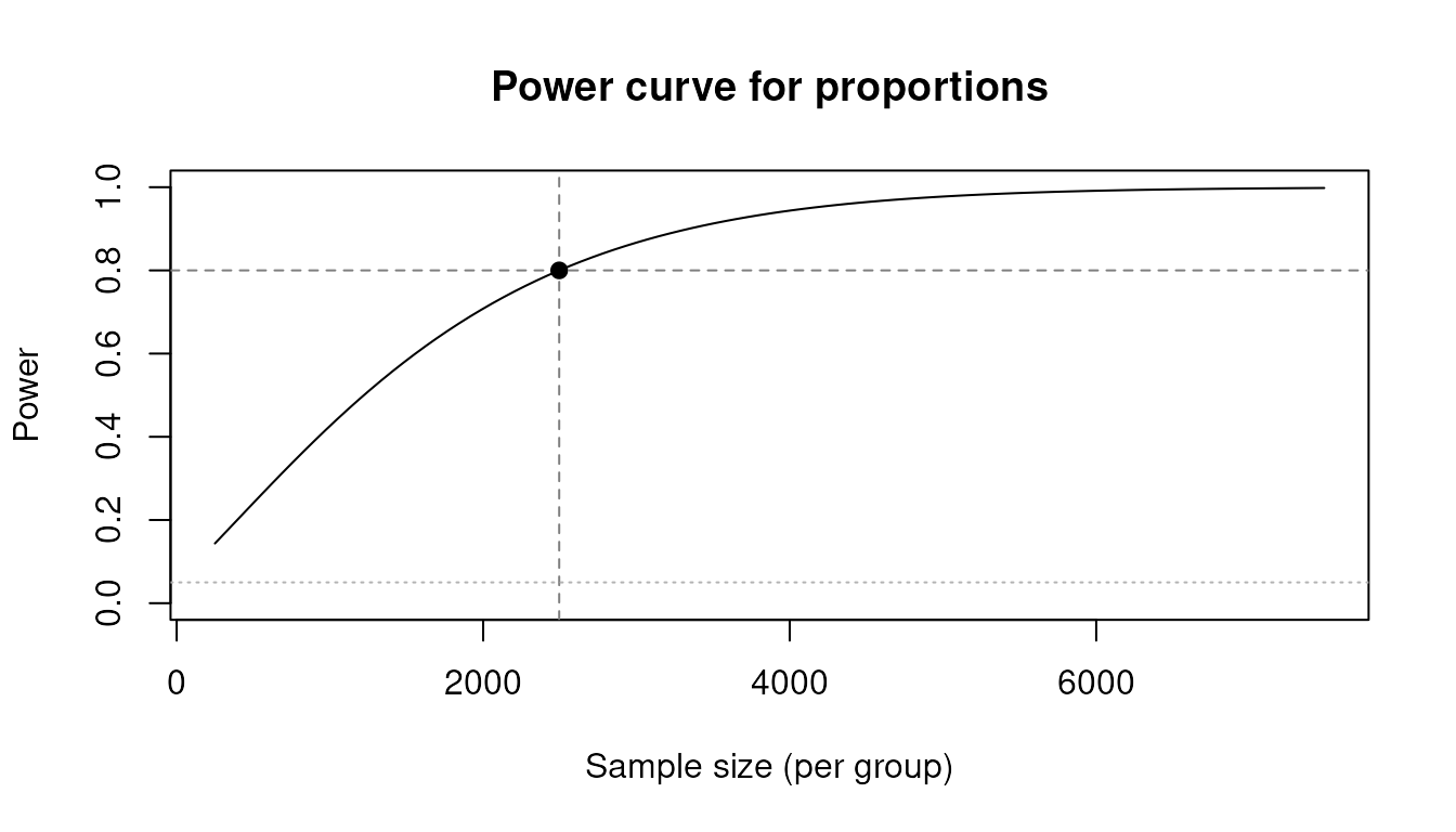

Sensitivity analysis

How sensitive is a sample size to assumptions about the design effect, response rate, or prevalence? The predict() method evaluates any svyplan result at new parameter combinations.

Varying design parameters

x <- n_prop(p = 0.3, moe = 0.05, deff = 1.5)
predict(x, expand.grid(
  deff = c(1.0, 1.5, 2.0, 2.5),
  resp_rate = c(0.8, 0.9, 1.0)
))
#>    deff resp_rate         n         se  moe         cv      rmoe
#> 1   1.0       0.8  403.3532 0.02551067 0.05 0.08503558 0.1666667
#> 2   1.5       0.8  605.0298 0.02551067 0.05 0.08503558 0.1666667
#> 3   2.0       0.8  806.7064 0.02551067 0.05 0.08503558 0.1666667
#> 4   2.5       0.8 1008.3829 0.02551067 0.05 0.08503558 0.1666667
#> 5   1.0       0.9  358.5362 0.02551067 0.05 0.08503558 0.1666667
#> 6   1.5       0.9  537.8042 0.02551067 0.05 0.08503558 0.1666667
#> 7   2.0       0.9  717.0723 0.02551067 0.05 0.08503558 0.1666667
#> 8   2.5       0.9  896.3404 0.02551067 0.05 0.08503558 0.1666667
#> 9   1.0       1.0  322.6825 0.02551067 0.05 0.08503558 0.1666667
#> 10  1.5       1.0  484.0238 0.02551067 0.05 0.08503558 0.1666667
#> 11  2.0       1.0  645.3651 0.02551067 0.05 0.08503558 0.1666667
#> 12  2.5       1.0  806.7064 0.02551067 0.05 0.08503558 0.1666667

Cluster budget scenarios

cl <- n_cluster(stage_cost = c(500, 50), icc = 0.05, budget = 100000)
predict(cl, data.frame(budget = c(50000, 100000, 150000, 200000)))
#>   budget     n_psu n_per_psu   total_n         cv   cost
#> 1  50000  42.04499  13.78405  579.5501 0.05318275  50000
#> 2 100000  84.08997  13.78405 1159.1003 0.03760588 100000
#> 3 150000 126.13496  13.78405 1738.6504 0.03070507 150000
#> 4 200000 168.17994  13.78405 2318.2006 0.02659137 200000

Power curves

pw <- power_prop(p1 = 0.30, p2 = 0.35, n = 500, power = NULL)
predict(pw, data.frame(n = seq(200, 1000, 200)))
#>      n     power effect
#> 1  200 0.1877131   0.05
#> 2  400 0.3272968   0.05
#> 3  600 0.4569385   0.05
#> 4  800 0.5707088   0.05
#> 5 1000 0.6665884   0.05

Precision by sample size

pr <- prec_prop(p = 0.3, n = 400)
predict(pr, data.frame(n = c(100, 200, 400, 800, 1600)))
#>      n         se        moe         cv       rmoe
#> 1  100 0.04582576 0.08981683 0.15275252 0.29938944
#> 2  200 0.03240370 0.06351009 0.10801234 0.21170031
#> 3  400 0.02291288 0.04490842 0.07637626 0.14969472
#> 4  800 0.01620185 0.03175505 0.05400617 0.10585015
#> 5 1600 0.01145644 0.02245421 0.03818813 0.07484736

Putting it all together

A typical planning sequence for a national household survey ties several svyplan functions together. A svyplan() profile captures the shared design assumptions:

1. Set shared design parameters once with svyplan()
2. Define indicators and precision targets per domain
3. Compute sample sizes with n_multi()
4. Evaluate achieved precision with prec_multi()
5. Run sensitivity analysis with predict()
6. If frame data is available, estimate variance components with varcomp()
7. Optimize the multistage allocation with n_cluster() or n_multi_cluster()
8. Determine strata boundaries with strata_bound()
9. Check that the design has adequate power with power_prop() / power_mean()

# 1: shared design assumptions
design <- svyplan(deff = 2.0, resp_rate = 0.85)

# 2-3: multi-indicator sample size
targets <- data.frame(
  name = c("stunting", "vaccination", "anemia"),
  p    = c(0.25, 0.70, 0.12),
  moe  = c(0.05, 0.05, 0.03),
  deff = c(2.0, 1.5, 2.5)
)
result <- n_multi(targets)
result
#> Multi-indicator sample size
#> n = 1127 (binding: anemia)
#> 
#>  name        .n   .cv_target .cv_achieved .binding
#>  stunting     577 0.10204269 0.07297042           
#>  vaccination  485 0.03644382 0.02388518           
#>  anemia      1127 0.12755336 0.12755336   *

# 4: achieved precision for each indicator
prec_multi(result)
#> Multi-indicator sampling precision
#> 
#>  name        .se        .moe .rmoe      .cv       
#>  stunting    0.02551067 0.05 0.20000000 0.10204269
#>  vaccination 0.02551067 0.05 0.07142857 0.03644382
#>  anemia      0.01530640 0.03 0.25000000 0.12755336

# 5: how sensitive is the binding indicator to the response rate?
predict(
  n_prop(p = 0.25, moe = 0.05, plan = design),
  data.frame(resp_rate = c(0.7, 0.8, 0.9, 1.0))
)
#>   resp_rate        n         se  moe        cv rmoe
#> 1       0.7 823.1697 0.02551067 0.05 0.1020427  0.2
#> 2       0.8 720.2735 0.02551067 0.05 0.1020427  0.2
#> 3       0.9 640.2431 0.02551067 0.05 0.1020427  0.2
#> 4       1.0 576.2188 0.02551067 0.05 0.1020427  0.2

# 9: can we detect a 5pp decline in stunting with this sample?
power_prop(
  p1 = 0.25, p2 = 0.20,
  n = as.integer(result), power = NULL,
  plan = design
)
#> Power analysis for proportions (solved for power)
#> n = 1127 (net: 958, per group), power = 0.459, effect = 0.0500
#> (p1 = 0.250, p2 = 0.200, alpha = 0.05, deff = 2.00, resp_rate = 0.85)

Sample-size, cluster, power, and strata-boundary results support as.integer() and as.double(). For sample-size results, these return the rounded-up and exact values of n, respectively, which makes it straightforward to pass results between functions or into other packages.

Scope

svyplan answers one question in several forms: how many units does a planned design need, and what precision does a given design achieve. Some neighbouring topics are deliberately outside that boundary. They are listed here so their absence reads as a decision rather than an oversight.

Totals. There is no n_total(). A total is a mean rescaled by N, so the CV target is identical and a margin of error on the total is moe / N on the mean. ?n_mean has a worked section on sizing for a total.

Ratio and regression estimation. Ratio estimators and regression estimators are analysis-stage techniques. Designs are not usually sized around the precision of a ratio, and sizing for a regression coefficient is a general statistical problem rather than a survey one, covered by packages such as pwr. The survey-specific part, the variance inflation from a complex design, is already the deff argument.

Two-phase designs beyond stratification and follow-up. n_twophase() allocates a two-phase sample: a large cheap phase 1, then a subsample measured on the expensive variable. Double sampling for stratification and nonresponse follow-up are the same problem in that function, differing only in which strata are marked take_all. What is not covered is the third member of the family, double sampling for a regression or ratio estimator, where the phase-1 variable is continuous rather than a stratifier. Its variance effect is expressible today as a design effect below 1, since a regression estimator multiplies the variance by $1 - \rho^2$, but the cost trade-off between the phases is not built in.

More than three stages. Two- and three-stage designs are supported. Surveys rarely go deeper, and the cost and variance models for a fourth stage would carry more assumptions than they would earn.

Attrition, and choosing a rotation. n_panel() is arithmetic on declared rates. It says what recruitment yields under a response rate and a retention curve, not where those rates come from. Attrition modelling, attrition weighting, and any adjustment for informative dropout are analysis-stage work and outside the boundary. Two consequences are worth stating. A unit lost at one wave is treated as lost for good, so a panel whose nonrespondents return later does better than planned here, and planning this way over-issues. Also, design_overlap() reads a schedule that has already been chosen. It does not solve the inverse problem of finding a schedule that delivers a target overlap while limiting how many times a unit may be interviewed.

Targeting nonresponse follow-up. Deciding how much follow-up to do is answered by n_twophase(). Deciding which cases to pursue is not, and is out of scope: prioritizing by response propensity, or adapting effort as fieldwork proceeds, needs paradata from the field that no planning stage has.

PPS selection inside joint allocation. varcomp() estimates variance components under PPS first-stage selection, but the joint allocator (n_alloc() with measures and targets) optimizes a variance written for equal-probability PSU selection. Feeding it components estimated under PPS is therefore an approximation, and the more unequal the sizes, the rougher it is.

Certainty units are better supported than that might suggest. strata_bound(take_all_above = ) cuts a census stratum at a size threshold, and a take_all frame column makes n_alloc() enumerate that stratum, in joint mode as much as in any other. What is genuinely unavailable is take_all in a fixed-take multistage joint design, where it is refused rather than approximated: taking every PSU still leaves a sample of units within each one, so it does not establish the ultimate-unit census that take_all asserts. A certainty PSU stratum in a multistage design is thus the case you construct yourself, by splitting the frame on the measure of size and planning that stratum separately.

Domains not identifiable on the frame. Targets can be set per domain when domain membership is known before fielding, as it is for region or urban/rural. For domains realized only after contact, such as age or sex subgroups, the realized subsample is random and has to be inflated by hand from the expected domain share. The same line runs through design_df(): a domain that is a union of whole strata gets an exact degrees-of-freedom count in $domains, while one cutting across strata does not, because counting the PSUs that contain its members needs frame information a plan does not carry.

Converting between listing units and analysis units. Sizing works in the units the precision target refers to. Converting a size in eligible persons to a number of households to list, given a mean household size and an eligibility rate, is arithmetic the user does explicitly. The MICS/DHS section above and the README both show the calculation.