Allocation, domains, and two-phase designs • svyplan

This article covers multi-indicator requirements, stratification, constrained allocation, and two-phase sampling. Start with Getting started, or continue with multistage planning, repeated surveys, and power and sensitivity.

Multi-indicator surveys

Household surveys like the Demographic and Health Surveys (DHS) or MICS track many indicators simultaneously. Each indicator has its own expected prevalence, precision target, and design effect. n_multi() finds the sample size that satisfies all targets at once.

targets <- data.frame(
  name = c("stunting", "vaccination", "anemia"),
  p    = c(0.25, 0.70, 0.12),
  moe  = c(0.05, 0.05, 0.03),
  deff = c(2.0, 1.5, 2.5)
)

n_multi(targets)
#> Multi-indicator sample size
#> n = 1127 (binding: anemia)
#> 
#>  name        .n   .cv_target .cv_achieved .binding
#>  stunting     577 0.10204269 0.07297042           
#>  vaccination  485 0.03644382 0.02388518           
#>  anemia      1127 0.12755336 0.12755336   *

The binding indicator (marked with *) drives the overall sample size. The other indicators are estimated with better precision than requested.

Proportion rows accept the same four methods as n_prop(), either for the whole table through prop_method or per row through a prop_method column. A df column sets each row’s interval quantile, so one table can mix an ordinary indicator with a rare one estimated from few clusters:

targets_rare <- data.frame(
  name = c("stunting", "cocaine_use"),
  p    = c(0.25, 0.02),
  moe  = c(0.05, 0.01),
  prop_method = c("wald", "beta"),
  df   = c(NA, 25)
)

n_multi(targets_rare)
#> Multi-indicator sample size
#> n = 949 (binding: cocaine_use)
#> 
#>  name        .n  .cv_target .cv_achieved .binding
#>  stunting    289 0.1020427  0.05625071           
#>  cocaine_use 949 0.2273345  0.22733454   *

Achieved precision

prec_multi() computes the achieved precision for each indicator at the chosen n:

plan <- n_multi(targets)
prec_multi(plan)
#> Multi-indicator sampling precision
#> 
#>  name        .se        .moe .rmoe      .cv       
#>  stunting    0.02551067 0.05 0.20000000 0.10204269
#>  vaccination 0.02551067 0.05 0.07142857 0.03644382
#>  anemia      0.01530640 0.03 0.25000000 0.12755336

Domain targets

Surveys often need adequate precision within subpopulations (urban/rural, regions). Add domain columns to the targets data frame and n_multi() optimizes each domain separately:

targets_dom <- data.frame(
  name       = rep(c("stunting", "vaccination", "anemia"), each = 2),
  residence  = rep(c("urban", "rural"), 3),
  p          = c(0.18, 0.32, 0.80, 0.60, 0.08, 0.16),
  moe        = c(0.05, 0.05, 0.05, 0.05, 0.03, 0.03),
  deff       = c(1.5, 2.5, 1.2, 1.8, 2.0, 3.0)
)

n_multi(targets_dom, domains = "residence")
#> Multi-indicator sample size (2 domains, separate quotas)
#> n = 2350 (sum of domain quotas)
#> Largest single domain = 1721 (binding: anemia)
#> 
#>  residence .n   .binding
#>  urban      629 anemia  
#>  rural     1721 anemia

Domain columns are specified explicitly via the domains parameter, and domain_sampling decides how the per-domain requirements combine into the single n that is reported. The default "separate" treats the domains as disjoint quotas drawn independently, the usual case for regional domains in one national survey, and reports their sum: every quota has to be met, so nothing smaller delivers the design. "natural" treats them as analytic domains arising at their own rate inside one sample, requires a share column, and reports max(.n / share), the size whose expected yield meets every quota.

Neither reading is the largest single domain requirement. That number is reported separately as n_domain_max, and it is what binding refers to. Use $domains to see each domain’s own sample size.

Relative precision in MICS and DHS

MICS is a household survey program run by UNICEF, and DHS is one funded by USAID and implemented by ICF. Both run standardized questionnaires and sample designs across many countries so that indicators on children, women, health and nutrition stay comparable across borders, and both publish the sampling rules their country teams work to. Those rules are where a planner meets the two relative precision targets in this package, and the two programs do not use the same one.

MICS states a requirement as a relative margin of error, the margin of error as a fraction of the indicator, which is what rmoe takes. DHS states one as a relative standard error, the standard error over the indicator, which its sampling manual also calls the coefficient of variation and which is what cv takes. They are not interchangeable. Under Wald, rmoe = q * cv, where q is the normal quantile by default and the t quantile when df is supplied. The identity does not hold under the other interval methods. rmoe is available on the scalar functions and as an indicator column.

The sampling rules are published. UNICEF’s MICS tools carry the sample size template for the current MICS7 round, and the DHS rules are in ICF International (2012), Demographic and Health Survey Sampling and Household Listing Manual, Calverton, Maryland (PDF).

rmoe is moe / p, so it fixes the same interval moe does while scaling with the estimate the way cv does. That places the package’s four precision quantities on two axes: se and cv describe the sampling variance, while moe and rmoe describe the interval drawn around it.

	Absolute	Relative
Sampling	`se`	`cv`
Interval	`moe`	`rmoe`

The sampling row is free of alpha and of the interval method, whereas the interval row depends on both. A rare outcome shows the split at its widest:

sapply(c("wald", "wilson", "logodds", "beta"), function(m) {
  r <- prec_prop(p = 0.02, n = 900, deff = 2, df = 25, method = m)
  c(se = r$se, cv = r$cv, moe = r$moe, rmoe = r$rmoe)
})
#>             wald      wilson     logodds        beta
#> se   0.006599663 0.006599663 0.006599663 0.006599663
#> cv   0.329983165 0.329983165 0.329983165 0.329983165
#> moe  0.013592261 0.014251833 0.014565337 0.014997984
#> rmoe 0.679613049 0.712591665 0.728266856 0.749899196

se and cv do not move across the four columns, but moe and rmoe do. So rmoe = q * cv, where q is the interval quantile the design uses (qnorm(1 - alpha / 2), or the t quantile on df degrees of freedom when df is supplied, as here), holds under Wald alone. Under the other three, reading a relative margin of error off the CV that way overstates the precision by 5 to 10 percent in this design, which is why a relative margin of error is a target in its own right rather than a rescaled cv.

# MICS-style: 12% relative MOE per domain, domain-specific deff and prevalence
targets_mics <- data.frame(
  name      = rep(c("stunting", "vaccination"), each = 3),
  region    = rep(c("North", "Central", "South"), 2),
  p         = c(0.35, 0.25, 0.40, 0.60, 0.75, 0.55),
  rmoe      = 0.12,
  deff      = c(2.5, 2.0, 3.0, 1.5, 1.2, 1.8),
  resp_rate = c(0.90, 0.85, 0.95, 0.90, 0.85, 0.95)
)

n_multi(targets_mics, domains = "region")
#> Multi-indicator sample size (3 domains, separate quotas)
#> n = 4523 (sum of domain quotas)
#> Largest single domain = 1884 (binding: stunting)
#> 
#>  region  .n   .binding
#>  North   1377 stunting
#>  Central 1884 stunting
#>  South   1264 stunting

The MICS template reports sample size in households. svyplan returns the number of individuals in the target population. To convert, divide by the expected number of eligible individuals per household: n_hh = ceiling(n / (pb * hh_size)), where pb is the share of the target population in the total population and hh_size is the average household size.

Minimum sample size per domain

The min_n_domain parameter sets a floor for the per-domain sample size (n_alloc() uses min_n_stratum for its per-stratum floor):

n_multi(targets_dom, domains = "residence", min_n_domain = 300)
#> Multi-indicator sample size (2 domains, separate quotas, min_n_domain = 300)
#> n = 2350 (sum of domain quotas)
#> Largest single domain = 1721 (binding: anemia)
#> 
#>  residence .n   .binding
#>  urban      629 anemia  
#>  rural     1721 anemia

Mixing proportions and means

Targets can mix proportion and mean indicators. Use var and mu columns for means (leave p as NA), and p for proportions (leave var/mu as NA):

targets_mixed <- data.frame(
  name = c("vaccination", "expenditure"),
  p    = c(0.70, NA),
  var  = c(NA, 40000),
  mu   = c(NA, 800),
  cv   = c(0.05, 0.10),
  deff = c(1.5, 2.0)
)

n_multi(targets_mixed)
#> Multi-indicator sample size
#> n = 258 (binding: vaccination)
#> 
#>  name        .n  .cv_target .cv_achieved .binding
#>  vaccination 258 0.05       0.05000000   *       
#>  expenditure  13 0.10       0.02204793

Strata boundaries

When a continuous auxiliary variable is available on the frame, strata_bound() constructs cut points intended to reduce the sample size or CV for a given number of strata. The iterative choices below are local heuristics, so their result is a candidate solution rather than a certified global minimum.

The boundaries are built from the distribution of x alone, and the variance they minimize is that of the total or mean of x. Nothing models the study variable’s conditional mean or variance given x, so for any y other than x the result is a proxy, good in proportion to how closely y tracks x. The reported CV is likewise the CV for x. Stratifying an expenditure frame to measure a poverty rate is the case this serves well, whereas stratifying on a variable unrelated to the indicator is not.

set.seed(12345)
x <- rlnorm(5000, meanlog = 6, sdlog = 1.2)

strata_bound(x, n_strata = 4, n = 300, method = "cumrootf")
#> Strata boundaries (Dalenius-Hodges, 4 strata)
#> n = 300, cv = 0.0199, allocation: neyman
#> 
#>  stratum  lower upper    N share     sd   mean   n
#>        1 3.8267   400 2473 0.495  105.3  191.4  48
#>        2    400  1200 1647 0.329  222.7  700.6  68
#>        3   1200  3100  672 0.134  519.5 1871.7  65
#>        4   3100 21958  208 0.042 3094.3 5543.6 119

Four methods are available:

Method	Algorithm	Speed	Best for
`"cumrootf"`	Dalenius-Hodges cumulative root frequency	Fast	General use
`"geo"`	Geometric progression	Fast	Skewed data
`"lh"`	LH-inspired coordinate optimization	Moderate	Fast local search
`"kozak"`	Kozak-inspired random-restart local search	Slow	More starting points

The "kozak" heuristic explores multiple starts and can find a better local solution on highly skewed distributions. Neither iterative method guarantees a global optimum or claims to reproduce the published algorithm exactly:

strata_bound(x, n_strata = 4, cv = 0.05, method = "kozak")
#> Strata boundaries (Kozak-inspired local search, 4 strata)
#> n = 60, cv = 0.0496, allocation: neyman
#> 
#>  stratum  lower  upper    N share     sd   mean  n
#>        1 3.8267 407.85 2503 0.501  107.2  194.0 10
#>        2 407.85 1227.1 1644 0.329  228.5  714.5 14
#>        3 1227.1 3447.4  682 0.136  587.1 1973.4 15
#>        4 3447.4  21958  171 0.034 3206.8 6036.3 21

Allocation methods

Allocation within strata is controlled by the alloc parameter:

"proportional": n_h \propto N_h
"neyman" (default): n_h \propto N_h \cdot S_h (minimizes national CV)
"optimal": n_h \propto N_h \cdot S_h / \sqrt{c_h} (accounts for costs)
"power": Bankier (1988) compromise, n_h \propto S_h \cdot N_h^{q}, where the exponent alloc_q \in [0, 1] controls the trade-off between national precision (alloc_q = 1, Neyman) and equal subnational CVs (alloc_q = 0)

# Bankier power allocation (compromise, alloc_q = 0.5)
strata_bound(x, n_strata = 4, n = 300, alloc = "power", alloc_q = 0.5)
#> Strata boundaries (LH-inspired coordinate search, 4 strata, converged)
#> n = 300, cv = 0.0216, allocation: power (alloc_q = 0.50)
#> 
#>  stratum  lower  upper    N share     sd   mean   n
#>        1 3.8267 456.28 2710 0.542  120.7  212.0  34
#>        2 456.28   1351 1529 0.306  244.5  787.5  52
#>        3   1351 4330.7  650 0.130  743.3 2243.4 103
#>        4 4330.7  21958  111 0.022 3441.5 7218.5 111

Classifying new observations

predict() applies the learned boundaries to new data, returning a factor:

sb <- strata_bound(x, n_strata = 4, n = 200, method = "cumrootf")
new_x <- c(100, 500, 1500, 5000)
predict(sb, newdata = new_x, labels = paste0("S", 1:4))
#> [1] S1 S2 S3 S4
#> Levels: S1 S2 S3 S4

Visualizing allocation

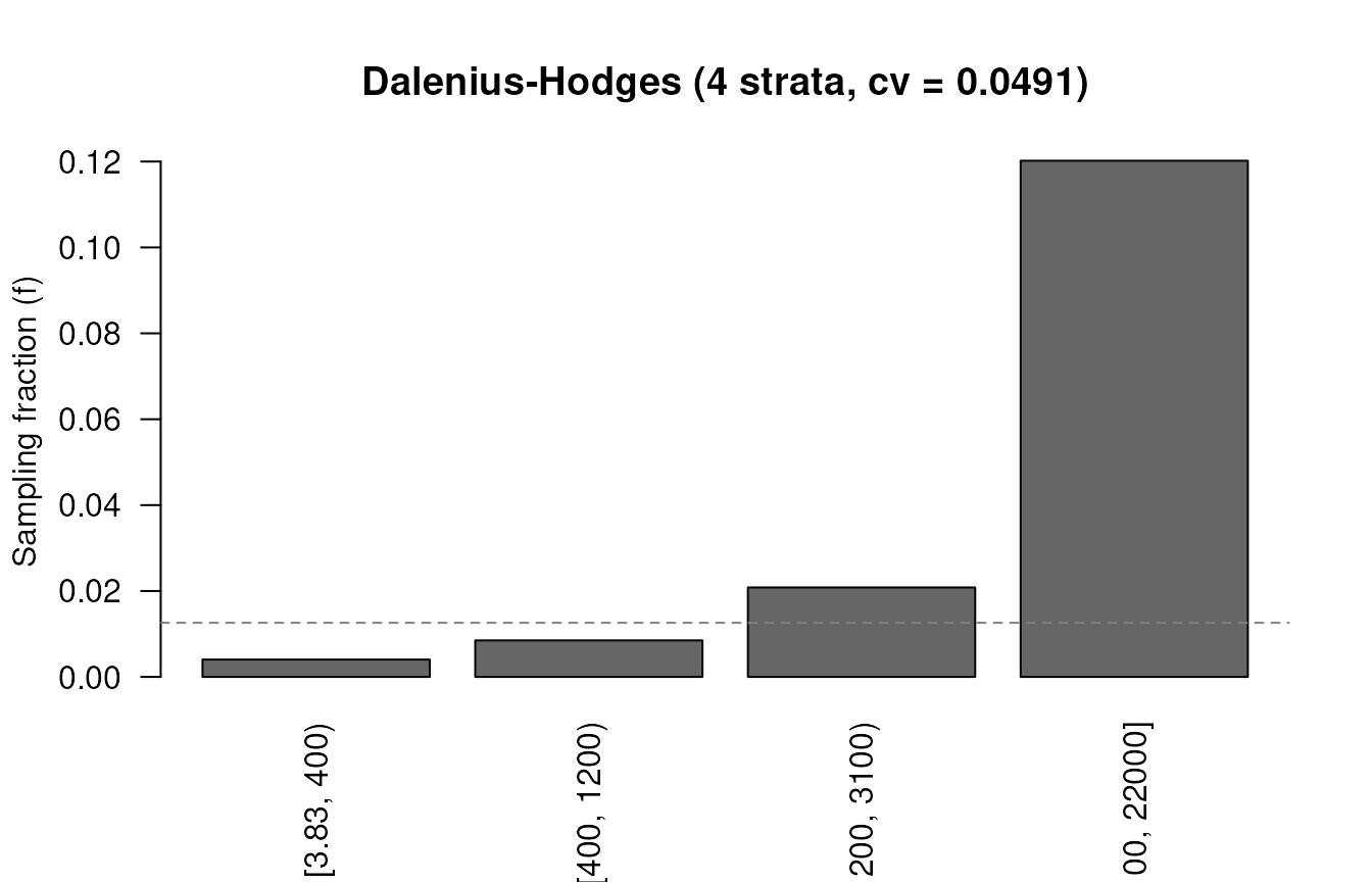
plot() shows the sampling fraction per stratum. Under Neyman allocation, high-variance strata are sampled more intensively. The dashed line marks the overall fraction:

plot(sb)

Handing boundaries to the allocator

$strata carries the N, sd, and mean columns n_alloc() needs, so the two halves of a stratified design connect directly:

sb_cv <- strata_bound(x, n_strata = 4, cv = 0.05, method = "lh")
n_alloc(sb_cv$strata, cv = 0.05)
#> Stratum allocation (neyman, 4 strata)
#> field design: n = 59, cv = 0.0490, cost = 59
#> continuous optimum: n = 56.83406, cv = 0.0500, se = 40.3814
#> (deff = 1)
#> design df = 55

Both functions evaluate the same variance, so cv means the same thing to each and n is a fielded sample in both. Design assumptions carry across unchanged, whether passed directly or through a svyplan() profile:

plan <- svyplan(deff = 1.8, resp_rate = 0.85)
sb_deff <- strata_bound(x, n_strata = 4, cv = 0.05, plan = plan)
sb_deff$n
#> [1] 118
n_alloc(sb_deff$strata, cv = 0.05, plan = plan)$n
#> [1] 116.4124

The remaining gap between the two totals is integer rounding, not a difference in model: strata_bound() reports the whole-unit allocation in $strata$n, while n_alloc() reports the continuous optimum.

A scalar deff does not move the cut points. It scales the variance of every candidate boundary set equally, so what it changes is the n a target requires, not where the strata divide.

Stratified allocation

Given a sampling frame with stratum population sizes (N) and stratum standard deviations (sd), n_alloc() distributes a total sample across strata. This is the second half of a stratified design: strata_bound() finds the cut points, and n_alloc() allocates within strata.

frame <- data.frame(
  N = c(4000, 3000, 3000),
  sd = c(10, 15, 8),
  mean = c(50, 60, 55)
)

# Fixed total n with Neyman allocation
n_alloc(frame, n = 600, alloc = "neyman")
#> Stratum allocation (neyman, 3 strata)
#> field design: n = 600, cv = 0.0079, cost = 600
#> continuous optimum: n = 600, cv = 0.0079, se = 0.4305
#> (deff = 1)
#> design df = 597

Three solve modes are available: fixed total n, target cv, or budget constraint (when unit_cost is provided in the frame).

Constraints and domain-level targets are often the more practical use cases:

frame_constraints <- transform(
  frame,
  unit_cost = c(1, 1.5, 1),
  max_weight = c(25, 20, NA),
  take_all = c(FALSE, FALSE, TRUE)
)

n_alloc(frame_constraints, budget = 3500, alloc = "optimal", min_n_stratum = 40)
#> Stratum allocation (optimal, 3 strata)
#> field design: n = 3403, cv = 0.0076, cost = 3500
#> continuous optimum: n = 3403.425, cv = 0.0076, se = 0.4125
#> (min_n_stratum = 40, deff = 1)
#> design df = 401

frame_domains <- data.frame(
  province = c("North", "North", "South", "South"),
  stratum = c("Urban", "Rural", "Urban", "Rural"),
  N = c(2000, 3000, 1800, 3200),
  sd = c(12, 18, 10, 16),
  mean = c(55, 48, 58, 50)
)

# Minimum total n such that each province meets the CV target
n_alloc(frame_domains, domains = "province",
        cv = 0.04, alloc = "power", alloc_q = 0.3)
#> Stratum allocation (power, 4 strata)
#> field design: n = 112, cv = 0.0270, cost = 112
#> continuous optimum: n = 110.7422, cv = 0.0272, se = 1.4076
#> (deff = 1)
#> design df = 108
#> Domains: 2
#> 
#>  province .domain .n       .se      .moe     .rmoe      .cv    .cost
#>  North    5_North 59.23404 2.032000 3.982647 0.07839856 0.0400 59   
#>  South    5_South 51.50815 1.948447 3.818886 0.07221797 0.0368 52

prec_alloc() computes the achieved precision for any allocation:

prec_alloc(frame, n = c(200, 250, 150))
#> Sampling precision for alloc
#> n = 600 (3 strata)
#> se = 0.4321, moe = 0.8469, cv = 0.0079, rmoe = 0.0155

$detail carries the same numbers per stratum, so you can see where the precision is actually being bought. .share is the stratum’s contribution to the design variance of the overall mean and sums to 1:

prec_alloc(frame, n = c(200, 250, 150))$detail[, c("stratum", "n", ".se", ".cv", ".share")]
#>   stratum   n       .se        .cv    .share
#> 1       1 200 0.6892024 0.01378405 0.4070048
#> 2       2 250 0.9082951 0.01513825 0.3976329
#> 3       3 150 0.6366579 0.01157560 0.1953623

With domains, $domains reports the same table n_alloc() returns, so a design and its assessment compare row for row.

Fieldwork that differs across strata

deff and resp_rate take one value per stratum, either as vectors or as frame columns, for designs whose fieldwork is not uniform. A response rate that varies changes where the sample should go, not just how much of it comes back:

uneven <- data.frame(
  stratum   = c("Urban", "Peri-urban", "Rural"),
  N         = c(4000, 3000, 3000),
  sd        = c(10, 15, 8),
  mean      = c(50, 60, 55),
  resp_rate = c(0.92, 0.80, 0.65)
)
n_alloc(uneven, n = 600, alloc = "neyman")$detail[, c("stratum", "n", "n_int")]
#>      stratum        n n_int
#> 1      Urban 205.4620   205
#> 2 Peri-urban 247.8752   248
#> 3      Rural 146.6628   147

A value shared by every stratum is a constant factor that cancels out of a proportional weighting, so scalar deff and resp_rate behave exactly as before.

Joint indicator and domain targets

When one allocation must satisfy several estimands, use an atomic frame plus long measures and targets tables. Atomic means that every frame row has a single value for every domain classification in use. The example below crosses region and residence, allowing those two domain systems to overlap without requiring separate public functions or an alloc selector.

joint_frame <- data.frame(
  stratum = c("NU", "NR", "SU", "SR"),
  region = c("North", "North", "South", "South"),
  residence = c("Urban", "Rural", "Urban", "Rural"),
  N = c(1000, 2000, 1500, 1000),
  unit_cost = c(1, 1.2, 1.5, 1)
)

joint_measures <- data.frame(
  stratum = rep(joint_frame$stratum, 2),
  name = rep(c("vaccination", "income"), each = 4),
  p = c(0.50, 0.40, 0.60, 0.30, rep(NA, 4)),
  mean = c(rep(NA, 4), 50, 55, 60, 45),
  sd = c(rep(NA, 4), 10, 12, 15, 9)
)

joint_targets <- data.frame(
  name = c("vaccination", "vaccination", "income"),
  domain = c(".overall", "region", "residence"),
  level = c(NA, "North", "Urban"),
  cv = c(0.05, 0.08, NA),
  moe = c(NA, NA, 2)
)

joint_fit <- n_alloc(
  joint_frame,
  measures = joint_measures,
  targets = joint_targets,
  min_n_stratum = 2
)
joint_fit
#> Joint constrained allocation (Bethel)
#> question: cheapest design meeting every precision target
#> field design: n = 425, cost = 508 (3 targets, all pass)
#> continuous optimum: n = 424.8282, cost = 508 (integerizing costs +0.04%)
#> binding: vaccination@.overall:cv (target 0.05, achieved 0.05)
joint_fit$constraints
#>                    constraint        name    domain level .metric .target
#> 1     vaccination@.overall:cv vaccination  .overall  <NA>      cv    0.05
#> 2 vaccination@region=North:cv vaccination    region North      cv    0.08
#> 3  income@residence=Urban:moe      income residence Urban     moe    2.00
#>    .achieved    .ratio     .residual .tolerance        .se        .cv
#> 1 0.05000000 1.0000000  1.782579e-10      1e-06 0.02272727 0.05000000
#> 2 0.07030489 0.8788112 -1.211888e-01      1e-06 0.03046545 0.07030489
#> 3 1.85333281 0.9266664 -7.333360e-02      1e-06 0.94559534 0.01688563
#>         .moe      .rmoe .pass .binding .multiplier .sensitivity
#> 1 0.04454464 0.09799820  TRUE     TRUE  0.03000152    -18750.95
#> 2 0.05971119 0.13779506  TRUE    FALSE  0.00000000         0.00
#> 3 1.85333281 0.03309523  TRUE    FALSE  0.00000000         0.00

The optimizer minimizes variable cost subject to all three requirements. joint_fit$detail$n is the continuous optimum and joint_fit$detail$n_int is the deterministic feasible operational recommendation. The latter is locally cleaned but is not claimed to be a globally optimal integer solution. Both precision tables are retained:

prec_alloc(joint_fit)
#> Joint allocation precision (3 constraints)
#> targets: all pass
#> showing 1 binding of 3
#> 
#>  constraint              .metric .target .achieved .pass
#>  vaccination@.overall:cv cv      0.05    0.05      TRUE 
#> 
#> ... see $detail for all rows
prec_alloc(joint_fit, n = joint_fit$detail$n_int)
#> Joint allocation precision (3 constraints)
#> targets: all pass

A modified named allocation can be assessed in any order because names are matched exactly to frame$stratum.

The precision a joint allocation plans for can be checked against the precision it delivers, by executing the design repeatedly against a known population and comparing empirical CVs with $constraints$.achieved. Two things are worth fixing before reading such a check. Compare against $constraints$.achieved rather than against the target, since integerization leaves the realized design a little better than what was asked for, and set the acceptance band in advance from the number of replicates, since an empirical CV from a few hundred draws carries its own error. The recipe needs a sampling engine to execute the design, so it belongs with one rather than here.

Fixed-take multistage joint allocation

The same public interface supports two- and three-stage designs when every later-stage take is fixed. The frame owns stage populations, takes, and costs. The measures table owns indicator-specific stage homogeneity parameters. Only n_psu is optimized. Public n, planning bounds, and precision assessments remain in ultimate-unit units.

This three-stage example samples PSUs, then a fixed number of SSUs per PSU, then a fixed number of ultimate units per SSU:

joint_frame_3stage <- within(joint_frame, {
  unit_cost <- NULL
  N_psu <- c(100, 160, 120, 90)
  N_ssu <- c(600, 1200, 900, 500)
  n_per_psu <- c(8, 10, 12, 7)
  n_per_ssu <- c(4, 5, 3, 4)
  cost_psu <- c(300, 400, 450, 350)
  cost_ssu <- c(25, 30, 35, 28)
  cost_tsu <- c(5, 6, 7, 5)
})

joint_measures_3stage <- transform(
  joint_measures,
  icc_psu = rep(c(0.03, 0.05, 0.08, 0.04), 2),
  icc_ssu = rep(c(0.10, 0.08, 0.12, 0.06), 2),
  var_ratio_psu = 1,
  var_ratio_ssu = 1
)

joint_fit_3stage <- n_alloc(
  joint_frame_3stage,
  measures = joint_measures_3stage,
  targets = joint_targets,
  min_n_stratum = 20
)
joint_fit_3stage$detail[, c(
  "stratum", "n_psu_int", "n_per_psu", "n_per_ssu", "n_int"
)]
#>   stratum n_psu_int n_per_psu n_per_ssu n_int
#> 1      NU         6         8         4   192
#> 2      NR        11        10         5   550
#> 3      SU         9        12         3   324
#> 4      SR         5         7         4   140
prec_alloc(joint_fit_3stage, n = joint_fit_3stage$detail$n_int)
#> Joint allocation precision (3 constraints)
#> targets: all pass

The exact operational identity is n_int = n_psu_int * n_per_psu * n_per_ssu. The standard multistage forms use N_psu, while three-stage frames also require the stratum’s total N_ssu. Fixed takes must be whole numbers. take_all is unavailable because taking every PSU alone does not establish a census of ultimate units.

Certainty PSUs from a register

For a two-stage joint allocation, a PSU register can replace N_psu. It has one row per PSU with stratum and N, and its totals must match frame$N. The allocation identifies PSUs whose implied PPS inclusion probability reaches one. A certainty column can add PSUs to that part of the design.

certainty_frame <- joint_frame_3stage[, setdiff(names(joint_frame_3stage),
                                                  c("N_ssu", "n_per_ssu", "cost_tsu"))]
certainty_frame$N_psu <- NULL

psu_register <- do.call(rbind, lapply(seq_len(nrow(certainty_frame)), function(i) {
  N <- certainty_frame$N[i]
  size <- rep(10, 20)
  size[1] <- floor(N / 3)
  size[2] <- N - sum(size[-2])
  data.frame(stratum = certainty_frame$stratum[i], N = size)
}))

certainty_fit <- n_alloc(
  certainty_frame,
  measures = joint_measures_3stage[, setdiff(names(joint_measures_3stage),
                                              c("icc_ssu", "var_ratio_ssu"))],
  targets = joint_targets,
  psu = psu_register,
  min_n_stratum = 20
)
certainty_fit$detail[, c("stratum", "n_psu_certain", "n_psu_draw", "n_int")]
#>   stratum n_psu_certain n_psu_draw n_int
#> 1      NU             2          2    89
#> 2      NR             2          2   169
#> 3      SU             2          2   134
#> 4      SR             2          2    75

$psu carries the classification, threshold, and source for every PSU. The operational allocation uses whole takes in certainty PSUs and whole PSUs in the remainder. prec_alloc(certainty_fit) reproduces its precision exactly.

Stratified two-stage designs

Most household surveys stratify first and cluster within each stratum, sampling enumeration areas and then households. Adding a icc_psu column to the frame switches n_alloc() to this design. The per-stratum homogeneity can come straight from varcomp() with strata, whose output columns are named to match the frame:

set.seed(3)
listing <- data.frame(
  region = rep(c("North", "South"), each = 600),
  ea = rep(1:60, each = 20),
  income = rnorm(1200, rep(c(50, 70), each = 600), 15) +
    rep(rnorm(60, 0, 6), each = 20)
)
vc_region <- varcomp(income ~ ea, data = listing, strata = ~region)
vc_region
#> Variance components (2-stage, 2 strata)
#> 
#>  stratum sd      mean    icc_psu var_ratio_psu varb   varw   unit_relvar
#>  North   15.6736 51.1316 0.1056  1.0489        0.0104 0.0882 0.0940     
#>  South   16.0116 69.3691 0.1595  1.0479        0.0089 0.0469 0.0533

frame_2stage <- merge(
  data.frame(stratum = c("North", "South"), N = c(40000, 60000)),
  as.data.frame(vc_region)[, c("stratum", "sd", "mean", "icc_psu", "var_ratio_psu")],
  by = "stratum"
)
frame_2stage$cost_psu <- c(400, 550)
frame_2stage$cost_ssu <- c(45, 60)

res_2stage <- n_alloc(frame_2stage, cv = 0.02)
res_2stage
#> Stratum allocation (neyman, two-stage, 2 strata)
#> field design: n = 338, n_psu = 44, cv = 0.0197, cost = 40205
#> continuous optimum: n = 323.6245, cv = 0.0200, se = 1.2415
#> (deff = 1)
#> design df = 42
res_2stage$detail[, c("stratum", "n_int", "n_per_psu", "n_psu_int")]
#>   stratum n_int n_per_psu n_psu_int
#> 1   North   135  8.675795        15
#> 2   South   203  6.951041        29

Each stratum gets its cost-optimal cluster take (fix it instead with a n_per_psu column), and the PSU counts fall out of the element allocation. Budget mode, min_n_stratum, and max_weight work the same way here. take_all does not apply: taking every PSU leaves the within-PSU take in force, so it does not enumerate a stratum, and it is refused rather than half-honoured.

An N_psu column caps each stratum at the PSUs it actually has, both in the continuous allocation and in the whole-unit design. Without it the allocation can ask for more clusters than a stratum contains:

frame_bounded <- frame_2stage
frame_bounded$N_psu <- c(40, 900)

res_bounded <- n_alloc(frame_bounded, n = 3000)
res_bounded$detail[, c("stratum", "n_psu", "n_psu_int", "N_psu",
                       ".psu_frac", ".bound_source")]
#>   stratum    n_psu n_psu_int N_psu .psu_frac .bound_source
#> 1   North  40.0000        40    40 1.0000000         N_psu
#> 2   South 381.6649       379   900 0.4240721          <NA>

North holds only 40 enumeration areas, so its allocation stops there and .bound_source names the constraint that stopped it. Asking for precision the remaining PSUs cannot deliver is an error rather than a silent overshoot, and it says the ceiling came from PSU availability under a with-replacement first stage rather than from the population.

N_psu is a feasibility constraint only. It does not switch on a first-stage finite population correction, so precision still uses a with-replacement first stage and stays conservative when a design takes an appreciable share of the available PSUs. print() says so when that happens, and .psu_frac reports the share.

Two-phase designs

In a two-phase (or double) sample, phase 1 draws a large sample and measures a variable the frame does not carry, and phase 2 subsamples those units and measures the variable of interest on them. What phase 1 measures decides which design it is, a stratification variable giving double sampling for stratification and response status giving nonresponse follow-up. n_twophase() allocates both phases at once, either to reach a target CV or to minimize it under a fixed budget.

The frame is one row per phase-2 stratum, similarly to what is used in n_alloc() :

frame <- data.frame(
  stratum   = c("A", "B", "C", "D"),
  N         = c(3500, 2500, 2500, 1500),
  sd        = c(12, 25, 8, 40),
  mean      = c(40, 70, 35, 90),
  unit_cost = c(2, 5, 1, 9)
)

n_twophase(frame, phase1_cost = 1, budget = 50000)
#> Two-phase allocation (4 phase-2 strata)
#> field design: n_phase1 = 16924 | n_phase2 = 8094
#> cv = 0.0050, cost = 50000
#> 
#>  stratum share    sd unit_cost     nu n_int
#>        A 0.350 12.00      2.00 0.4154  2462
#>        B 0.250 25.00      5.00 0.5474  2316
#>        C 0.250  8.00      1.00 0.3917  1659
#>        D 0.150 40.00      9.00 0.6528  1657
#> 
#> single-phase is better here: n = 14085 at cv 0.0046, so skip phase 1
#> # summary() for the continuous optimum and the comparator

The nu column is the fraction of each phase-1 stratum carried forward. Its shape is Neyman-like, proportional to S_h/\sqrt{c_h}, but the overall scale is set by the between-stratum variance: the weaker the stratification, the closer every fraction moves to 1, meaning keep everything phase 1 found.

Two design effects, not one

Neither phase has to be a simple random sample, and the two carry separate design effects because they apply to different things. phase1_deff inflates the between-stratum component, the part phase 1 is responsible for. A deff column inflates each stratum’s within-stratum residual, the part phase 2 has to measure. single_deff describes the comparator, which need not be fielded like phase 2.

clustered <- transform(frame, deff = c(1.2, 2.5, 0.8, 1.7))

n_twophase(clustered, phase1_cost = 1, budget = 50000,
           phase1_deff = 2.2, single_deff = 2.9)
#> Two-phase allocation (4 phase-2 strata)
#> field design: n_phase1 = 17999 | n_phase2 = 7172
#> cv = 0.0070, cost = 50000
#> phase-1 deff = 2.20, single-phase deff = 2.90
#> 
#>  stratum share    sd unit_cost deff     nu n_int
#>        A 0.350 12.00      2.00 1.20 0.3068  1933
#>        B 0.250 25.00      5.00 2.50 0.5835  2626
#>        C 0.250  8.00      1.00 0.80 0.2362  1064
#>        D 0.150 40.00      9.00 1.70 0.5738  1549
#> 
#> single-phase alternative: n = 14085 at cv 0.0079, two-phase wins
#> # summary() for the continuous optimum and the comparator

Inflating the combined variance by one design effect instead would be a different and wrong model. The two also pull against each other, and the trap runs in the direction that looks attractive: a stratifier built purely from between-cluster structure shrinks the residual, lowering the stratum deff, but it makes the fitted values nearly constant within clusters and so drives phase1_deff up toward the cluster size. Under a clustered phase 1 that first term can dominate, and the design loses to a plain sample even though the residual design effect looks favorable.

Every result carries the single-phase comparison, because two-phase sampling is not always an improvement. Skipping phase 1 and measuring directly can be both cheaper and more precise when the screener costs too much or the stratifier predicts too little, and the print output says so when that happens.

Response rates

Both phases can lose sample to nonresponse, and the two enter separately. resp_rate is the phase-1 response or successful-classification rate, and a resp_rate column is the phase-2 completion rate in each stratum. Response divides its own component, exactly as the design effects do, so a stratum that responds poorly is subsampled differently rather than the whole design being inflated by one factor.

screened <- transform(frame, resp_rate = c(0.9, 0.7, 0.85, 0.6))

n_twophase(screened, phase1_cost = 1, budget = 50000, resp_rate = 0.8)
#> Two-phase allocation (4 phase-2 strata)
#> field design: n_phase1 = 16034 | n_phase2 = 7880
#> expected responding: n_phase1 = 12827 | n_phase2 = 6003
#> cv = 0.0059, cost = 50000
#> 
#>  stratum share    sd unit_cost resp     nu n_int n_resp
#>        A 0.350 12.00      2.00 0.90 0.3917  2198   1978
#>        B 0.250 25.00      5.00 0.70 0.5852  2346   1642
#>        C 0.250  8.00      1.00 0.85 0.3800  1523   1295
#>        D 0.150 40.00      9.00 0.60 0.7538  1813   1088
#> 
#> single-phase is better here: n = 14085 at cv 0.0046, so skip phase 1
#> # summary() for the continuous optimum and the comparator

Everything here counts units issued, so a cost quoted per completed interview has to be converted first: c_contact + resp_rate * c_complete. Issued and expected-responding counts are reported separately, because they are different quantities and neither is an effective sample size. There is no single effective size for a two-phase design, since the two variance components carry different design effects.

Phase 2 can only draw from what phase 1 managed to classify, so every subsampling fraction is capped at the phase-1 response rate.

One caveat worth stating plainly: dividing by a response rate assumes response is ignorable within the strata you supplied. That is a substantive claim about the strata, not a property of the arithmetic, and no sample size removes nonresponse bias. Where the assumption is uncomfortable, modeling the nonresponse as a follow-up phase is the alternative the design itself offers.

When the phase-1 sample is already fixed

Often it is. The screener has run, or phase 1 is an existing survey, a panel, or a listing operation sized by field capacity rather than by this design. Phone surveys built on a previous face-to-face round are the common case. Supply n_phase1 and the only decision left is how deep to subsample.

n_twophase(frame, phase1_cost = 1, budget = 50000, n_phase1 = 20000)
#> Two-phase allocation (4 phase-2 strata)
#> field design: n_phase1 = 20000 | n_phase2 = 7340
#> cv = 0.0051, cost = 50000
#> 
#>  stratum share    sd unit_cost     nu n_int
#>        A 0.350 12.00      2.00 0.3189  2232
#>        B 0.250 25.00      5.00 0.4202  2101
#>        C 0.250  8.00      1.00 0.3006  1504
#>        D 0.150 40.00      9.00 0.5011  1503
#> 
#> single-phase is better here: n = 14085 at cv 0.0046, so skip phase 1
#> # summary() for the continuous optimum and the comparator

The relative allocation is unchanged, because it is S_h\sqrt{d_{2h}/c_h} in every mode. What moves is the overall scale, now pinned by the budget left after paying for phase 1 rather than by the variance-cost trade-off. Since the optimizing choice of n_phase1 is the best member of this family, fixing it can only match or lose to leaving it free, and the difference is what a phase-1 size you did not choose is costing you.

Two things can go wrong, and both give a specific error. The budget may not reach phase 2 at all. Or a target CV may sit below the phase-1 variance floor: what that n_phase1 leaves when every classified unit is carried into phase 2, which is

\frac{1}{\mu}\sqrt{\frac{1}{n_a}\left(\frac{d_1A}{r_1} + \sum_h \frac{d_{2h}W_hS_h^2}{r_{2h}r_1}\right) - \frac{d_1A + \sum_h d_{2h}W_hS_h^2}{N}}.

The between-stratum term is the part already paid for by the phase-1 size. It is not the whole floor, though, because subsampling stops at the classification rate rather than at 1, so the phase-2 residual survives at \nu_h = r_1 and is added to it. The subtracted term is the finite population correction, and it is what makes the floor vanish at a census: with n_a = N and no losses the two halves cancel exactly. It carries the design effects, since those inflate an SRSWOR variance here as everywhere, but not the response rates, because measuring every unit removes all the variance while failing to reach some of them does not.

Whole units and assurance

$operational carries the field design in whole units, and it is what the printed block reports: every count there is a whole unit off the same solution, so the phase sizes, the stratum takes and the responding figures reconcile. Budget mode floors and then buys back units in order of variance reduction per unit cost, staying inside the budget. CV mode rounds up, overshooting precision rather than missing it. summary() sets the continuous optimum beside the fielded design and gives the single-phase comparator in full.

Planning at the expected respondent count leaves roughly half of all designs short. assurance reports the issue for which the required respondents arrive with at least that probability, from the binomial distribution of respondents:

screened <- transform(frame, resp_rate = c(0.9, 0.7, 0.85, 0.6))

n_twophase(screened, phase1_cost = 1, budget = 50000,
           resp_rate = 0.8, assurance = 0.90)
#> Two-phase allocation (4 phase-2 strata)
#> field design: n_phase1 = 16034 | n_phase2 = 7880
#> expected responding: n_phase1 = 12827 | n_phase2 = 6003
#> cv = 0.0059, cost = 50000
#> 
#>  stratum share    sd unit_cost resp     nu n_int n_resp
#>        A 0.350 12.00      2.00 0.90 0.3917  2198   1978
#>        B 0.250 25.00      5.00 0.70 0.5852  2346   1642
#>        C 0.250  8.00      1.00 0.85 0.3800  1523   1295
#>        D 0.150 40.00      9.00 0.60 0.7538  1813   1088
#> 
#> assured (0.90): issue n_phase1 = 16116 | n_phase2 = 8010 (cost 50761)
#> single-phase is better here: n = 14085 at cv 0.0046, so skip phase 1
#> # summary() for the continuous optimum and the comparator

If the assured phase-2 issue exceeds the pool phase 1 supplies, that is a signal to enlarge phase 1 rather than to over-issue.

Nonresponse follow-up

Following up a subsample of nonrespondents is the same allocation problem with two strata. The respondents are already measured, so they cost nothing more and are all kept, which is unit_cost = 0 with take_all = TRUE. Only the nonrespondents are subsampled:

theta <- 0.5   # phase-1 response rate

nrfu <- data.frame(
  stratum   = c("respondents", "nonrespondents"),
  N         = c(theta, 1 - theta),
  sd        = c(1, 1),
  unit_cost = c(0, 200),
  take_all  = c(TRUE, FALSE)
)

n_twophase(nrfu, phase1_cost = 50, budget = 100000,
           mu = 1, single_cost = 50 / theta)
#> Two-phase allocation (2 phase-2 strata)
#> field design: n_phase1 = 828 | n_phase2 = 707
#> cv = 0.0382, cost = 1e+05
#> 
#>         stratum share   sd unit_cost     nu n_int take_all
#>     respondents 0.500 1.00      0.00 1.0000   414        *
#>  nonrespondents 0.500 1.00    200.00 0.7071   293         
#> 
#> single-phase is better here: n = 1000 at cv 0.0316, so skip phase 1
#> # summary() for the continuous optimum and the comparator

The optimal follow-up fraction reduces to \sqrt{c_1/(c_2\theta)} here, the standard result. Two details matter in this configuration. single_cost: a unit_cost of 0 means “already measured”, not “free”, so the baseline for the comparison has to be named explicitly as the cost of one completed interview without follow-up. And resp_rate should stay at its default of 1, because here the strata are response status, so classification succeeds for every unit and setting a phase-1 rate as well would count the same loss twice.