{samplyr}

A tidy grammar for survey sampling design

Ahmadou Dicko, PhD

useR! 2026 / Warsaw / 06-09 July

How many beds sleep under a net in The Gambia?

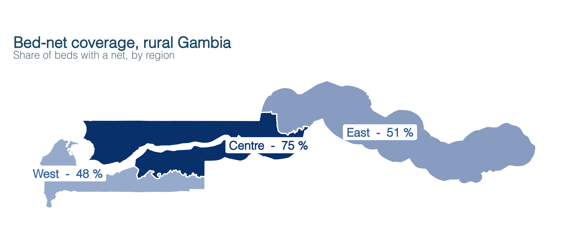
National survey in rural Gambia. D’Alessandro et al. (1994), Bull. WHO 72(3): 391–394.

We run the survey. Answer: ≈ 58 %

Malaria hits children first, and the insecticide-treated bed net is one of our cheapest tools.

Before a national programme, we need to know what share of the population sleeps under a net.

Two more questions steer the roll-out:

• How does coverage vary by region?
• It runs through local health centres, so do villages with one differ from those without?

Opening (1 min). Set the scene, a real public-health stake, the actual 1991 national survey. Three questions frame the survey. First, the overall share, answered by the 58 % reveal. Second, how it varies by region, the map already hints at it with the Centre standing out. Third, the health-centre comparison, paid off near the end at 59 % versus 58 %. The next slide is about how you get these numbers.

This is a textbook example

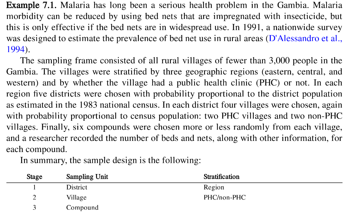
Sharon L. Lohr, Sampling: Design and Analysis, example 7.1.

D’Alessandro’s survey became example 7.1 in Lohr, a standard sampling textbook.

• Writing such a complex design in R tends to drift far from the plain description of the plan.
• To my surprise, the ones that stay closest are SAS PROC SURVEYSELECT and SPSS CSPLAN, whose dedicated survey-design syntax reads almost like the plan.
• Hence {samplyr}: express a design in R as plainly as you describe it.

1 min. Credit and motivation. The Gambian survey we follow throughout is example 7.1 in Lohr. The book and its R companion don’t ship SAS or SPSS code for this example. The tool comparison here is my own, more general observation, so don’t attribute it to Lohr. In practice, coding a multistage design like this in R drifts far from how the plan is described, whereas SAS PROC SURVEYSELECT reads close to the design, and SPSS CSPLAN, which I’ve seen used in national statistical offices, is more structured still. That gap, writing a design as plainly as you describe it, is what motivated samplyr.

Why not just base::sample()?

To express a design as plainly as we describe it, we first need to know what a design has to capture. On the ground, four constraints rule out that one-liner. The plan stays random all the way down, but it stops being simple, and each constraint names an idea.

• A figure per region, and by presence of a health centre -> strata
• Limit travel, cut costs -> group visits by village clusters
• No list of compounds available -> sample in stages stages
• A large village weighs more -> sample proportional to size PPS

Remember the colours. They follow us all the way to the code.

1.5 min. Brings in the vocabulary without formalism and sets up the colour code. The title’s answer: base::sample() is srswor, simple random sampling without replacement. The full plan is still random, every compound keeps a known probability of selection, it just stops being SIMPLE. And srswor does not go away, it is exactly stage 3 of the design, draw(n = 6). This is the Gambian design: six strata (region x health-centre presence), clusters drawn in batches, several stages, draws proportional to size. Each coloured badge reappears identically in the report, the diagram and the code.

The design, step by step

In 3 stages: 3 regions × 5 districts × 4 villages × 6 compounds = 360 visits. Bigger -> more likely to be drawn: that is PPS, probability proportional to size.

2 min. The draw as a story, one branch of the tree. The stacked cards behind each panel say it visually: this same card repeats, in each of the 3 regions, then each of the 15 chosen districts, then each of the 60 chosen villages. Each stage in two clicks: first the pool appears, then the draw happens, the winners pop in pink.

Regions: no draw at all, strata mean every region is guaranteed in.

Districts, click 1 the pool, click 2 the draw. Insist: in EVERY region we take five districts, not one. The raffle metaphor: a district with twice the people holds twice the tickets. Bigger circles, more likely pink. Point at the small pink one: small districts can still win, they just win less often.

Villages: inside every chosen district, villages come in two kinds, with a clinic and without. The blue dashed line splits them, and we pick 2 on EACH side, that is the comparison we promised at the start. Within each side, the same raffle again: larger villages, higher chance.

Compounds: once a village is chosen, the raffle stops. The die says it: purely at random, all dots identical, equal chance. That contrast IS the difference between PPS and simple random sampling.

Final line: in 3 stages, 3 x 5 x 4 x 6 = 360 compounds stand in for the whole country. Name the notion now that they have seen it twice: bigger, more likely, that is PPS, sampling proportional to size, the pink of the fil rouge. Do NOT talk about weights here, that comes with execute() later. Colours to anchor: blue guarantees coverage, orange draws whole groups, green counts the stages, pink is the size-proportional draw.

What the survey report says

The Gambian survey protocol, as published:

① Villages were stratified by region (East, Centre, West) and by presence of a health centre. In each region, five districts were drawn proportional to their population. ② In each district, four villages, again proportional to population. ③ Finally, six compounds were drawn in each village.

strata clusters stages PPS

1.5 min. The report on the left, the same structure as a diagram on the right. Read the protocol, follow the colours. Strata, clusters, stages, PPS: everything is already there, before a single line of code.

The same design in {sampling} and in SPSS

• SPSS CSPLAN
• {sampling}

* SPSS Complex Samples.
CSPLAN SAMPLE /PLAN FILE='gambia.csplan'
  /DESIGN STAGELABEL='districts'
    STRATA=region CLUSTER=district
  /METHOD TYPE=PPS_WOR
  /MOS VARIABLE=district_pop
  /SIZE VALUE=5
  /DESIGN STAGELABEL='villages'
    STRATA=phc CLUSTER=village
  /METHOD TYPE=PPS_WOR
  /MOS VARIABLE=village_pop
  /SIZE VALUE=2
  /DESIGN STAGELABEL='compounds'
   CLUSTER=compound_id
  /METHOD TYPE=SIMPLE_WOR
  /SIZE VALUE=6.

library(sampling)
# Stage 1: 5 districts per region, PPS (no Brewer here: systematic)
d <- unique(gmb_frame[c("region", "district", "district_pop")])
d <- d[order(d$region), ]
s1 <- strata(d, "region", size = rep(5, 3), method = "systematic",
             pik = d$district_pop)
# Stage 2: in each sampled district, 2 PHC + 2 non-PHC villages, PPS
v <- unique(gmb_frame[c("district", "phc", "village", "village_pop")])
v <- v[v$district %in% getdata(d, s1)$district, ]
v <- v[order(v$district, v$phc), ]
s2 <- strata(v, c("district", "phc"), size = rep(2, 30),
             method = "systematic", pik = v$village_pop)
# Stage 3: 6 compounds per sampled village (take all if fewer)
cpd <- gmb_frame[gmb_frame$village %in% getdata(v, s2)$village, ]
cpd <- cpd[order(cpd$village), ]
s3 <- strata(cpd, "village", size = pmin(6, table(droplevels(cpd$village))),
             method = "srswor")
# then getdata() three times, and compose the weights by hand...

SPSS keeps the plan closer to the description. In R using {sampling}, the stages become three hand-chained draws, and strata, clusters, sizes and probabilities are yours to keep aligned.

1.5 min. Two tabs, click to switch, we open on SPSS. CSPLAN reads like the protocol: one /DESIGN block per stage, with STRATA, CLUSTER and MOS, the colours are all there. But it lives outside R and the data pipeline.

Then the sampling tab. sampling is excellent on algorithms, but its multistage helper mstage cannot even express this design: stage 2 stratifies by district AND phc at once, which mstage has no way to say. So the realistic code is three strata() calls chained by hand: sort before each call, subset by the previous draw, no Brewer PPS (systematic instead), pmin for villages with fewer than 6 compounds, and the weights composed manually at the end. This code runs and gives 15 districts, 60 villages (30 PHC, 30 non), ~360 compounds. The coloured structure has vanished; the report describes a STRUCTURE, the code a sequence of operations. The more complex the design, the wider the gap, and probability errors are hard to catch.

We have solved this kind of gap before in R, with dplyr for data and ggplot2 for graphics. Grammars. samplyr makes the same bet for sampling: the readability of CSPLAN, inside R.

{samplyr}: the grammar follows the colours

The idea	In the report	In {samplyr}
Stratum	“stratified by region”	stratify_by(region)
Cluster	“five districts drawn together”	cluster_by(district)
Stage	“then, in each district…”	add_stage()
Sampling	“proportional to population”	draw(n, method, mos)

These four verbs describe the design. The weight is not written, it results from the design composed by execute() across the stages (.weight).

1.5 min. The correspondence slide. Four verbs for four design decisions: stratification, clusters, stages, and the sampling method (draw, including PPS). The weight is not a fifth verb, it is the result: draw sets unequal inclusion probabilities, execute() composes the weight across the three stages. draw is the sampling, not the weight.

Back to Gambia, the report and the code

① In each region, draw five districts proportional to population (PPS).

② In each district, by health centre, two villages PPS.

③ In each village, draw six compounds.

design <- sampling_design("Gambia bed nets") |>
  add_stage(label = "Districts") |>
    stratify_by(region) |>
    cluster_by(district) |>
    draw(n = 5, method = "pps_brewer",
         mos = district_pop) |>
  add_stage(label = "Villages") |>
    stratify_by(phc) |>
    cluster_by(village) |>
    draw(n = 2, method = "pps_brewer",
         mos = village_pop) |>
  add_stage(label = "Compounds") |>
    draw(n = 6)

The code mirrors the report, colour for colour, verb for verb.

2 min. The central slide, take your time. Each click brings up a sentence from the report on the left and the matching code block on the right, in the same colours. Read the sentence, then trace the cod e. A reviewer can check the code against the protocol without knowing the algorithmic details of Brewer PPS.

The design is a readable object

design

── Sampling Design: Gambia bed nets ────────────────

ℹ 3 stages

── Stage 1: Districts ──────────────────────────────
• Strata: region
• Cluster: district
• Draw: n = 5 (per stratum), method = pps_brewer, mos = district_pop

── Stage 2: Villages ───────────────────────────────
• Strata: phc
• Cluster: village
• Draw: n = 2 (per stratum), method = pps_brewer, mos = village_pop

── Stage 3: Compounds ──────────────────────────────
• Draw: n = 6, method = srswor

It shows the three stages, each with its strata, clusters and draw. Defined without any data so it can be reviewed and versioned before the frame exists.

glimpse(gmb_frame)

Rows: 19,344
Columns: 8
$ region       <fct> Eastern, Easter…
$ district     <fct> Eas-D01, Eas-D0…
$ phc          <fct> PHC, PHC, PHC, …
$ village      <fct> V0001, V0001, V…
$ compound_id  <int> 1, 2, 3, 4, 5, …
$ population   <int> 18, 19, 16, 19,…
$ district_pop <int> 9062, 9062, 906…
$ village_pop  <int> 506, 506, 506, …

The frame is synthetic, built to mirror the survey. It holds 19,344 compounds with their village and size, but no nets or beds yet.

0.5 min. The payoff of the grammar argument: the design is a first-class object. It prints legibly (three stages, each with its strata, clusters and draw method), documents and versions, and uses bare column names, so it can be written and validated during survey design, before the frame even exists. On the right, the frame it will meet: one row per compound, 19,344 of them, with region, village and size, but no nets. That is exactly what we go and measure. Say clearly that this frame is SYNTHETIC, built to mirror the real 1991 survey (D’Alessandro et al. 1994), so the 58 %/59 % we compute later are illustrative and land near the published figures by construction, not an independent re-analysis. Next slide, the two come together in execute().

Then we execute it, the design meets the frame

sample <- execute(design, gmb_frame, seed = 27)   # the design meets the frame
sample |> select(region, village, compound_id, phc, population, .weight)

# A tbl_sample: 360 × 6 | Gambia bed nets
# Weights:      53.65 [32.53, 77.69]
  region  village compound_id phc   population .weight
* <fct>   <fct>         <int> <fct>      <int>   <dbl>
1 Eastern V0007           242 PHC           22    60.5
2 Eastern V0007           224 PHC            8    60.5
3 Eastern V0007           236 PHC           27    60.5
4 Eastern V0007           241 PHC           19    60.5
5 Eastern V0007           234 PHC           22    60.5
# ℹ 355 more rows

execute() lists the 360 compounds to visit and already composes their weights across the three stages. But beds and nets are not there yet, and need to be collected on field.

1 min. Then execute() draws it: the tbl_sample comes out with the three-stage weights already composed, but WITHOUT the nets, the frame did not contain them. This is the realistic moment: we have the list of compounds to visit, we have not measured yet. execute() can also run stage by stage (stages =) to follow the field calendar.

From the field to the estimate

# back from visiting the 360 sampled compounds
sample <- sample |> left_join(terrain, join_by(compound_id))  # beds and nets measured on site
sample |> select(village, compound_id, nets, beds, .weight) |> slice_head(n = 3)

# A tbl_sample: 3 × 5 | Gambia bed nets
# Weights:      60.54 [60.54, 60.54]
  village compound_id  nets  beds .weight
* <fct>         <int> <int> <int>   <dbl>
1 V0007           242     6    18    60.5
2 V0007           224     4     9    60.5
3 V0007           236     0     4    60.5

svy <- as_svydesign(sample)        # samplyr to survey, everything filled in
r <- svyratio(~nets, ~beds, svy)   # share of protected beds
cbind(estimate = coef(r), confint(r))

          estimate     2.5 %    97.5 %
nets/beds 0.584394 0.5078807 0.6609073

There are the 58 % promised at the start, with a margin of error that accounts for the plan.

And the health-centre villages? Let’s use {srvyr} to find out

library(srvyr)
as_survey_design(sample) |>
  summarise(coverage = survey_ratio(nets, beds, vartype = "ci"), .by = phc)

# A tibble: 2 × 4
  phc     coverage coverage_low coverage_upp
  <fct>      <dbl>        <dbl>        <dbl>
1 PHC        0.591        0.504        0.678
2 non-PHC    0.577        0.465        0.689

59 % versus 58 %, almost identical. No marked coverage gap in villages without a health centre. The question we asked earlier now has its answer, with a margin of error.

1.5 min. Realism: nets are only measured on the compounds actually drawn, once on site. left_join attaches them. The weights do not move, they are a property of the design, not of what we observe. as_svydesign() fills strata, clusters, composed weights and FPC on its own. The protected-bed share comes out at 58 %, with the honest confidence interval, the one that accounts for the design structure, unlike a naive prop.test.

1 min. Paying off the promise from the step-by-step visual, where we drew as many rounds (PHC) as squares (non-PHC). Because we stratified by PHC, we have enough villages of both kinds to estimate each and compare. Result: 59 % vs 58 %, negligible gap given the standard errors. Policy conclusion: the programme does not leave out villages without a health centre. Exactly what the original report concluded.

Under the hood, nothing simplified

Sampling methods

• SRS, systematic, Bernoulli
• 8 PPS methods (Brewer, Pareto, Chromy…)
• Balanced sampling (cube)
• Custom methods (sondage::register_method())

Allocation and coordination

• Proportional, Neyman, optimal, power
• min_n / max_n bounds, PRN coordination

Migrating from SAS / SPSS

sampling_design() |>
  stratify_by(region) |>
  cluster_by(school) |>
  draw(n = 50, method = "pps_brewer",
       mos = enrollment) |>
  execute(frame, seed = 1)

* SAS proc surveyselect;
proc surveyselect data=frame
    method=PPS_SAMPFORD n=50 seed=1;
  strata region; cluster school;
  size enrollment;
run;

* SPSS Complex Sample
CSPLAN SAMPLE
  /DESIGN STRATA=region CLUSTER=school
  /METHOD TYPE=PPS_SAMPFORD
  /MOS VARIABLE=enrollment
  /SIZE VALUE=50.

Maps directly onto SAS PROC SURVEYSELECT (strata / cluster / size) and SPSS CSPLAN (STRATA / CLUSTER / MOS).

1 min. Credibility slide, go quickly. Message: samplyr is not a teaching toy, it is the full public-statistics arsenal behind a readable syntax. And many offices still run on SAS or SPSS, partly for lack of a readable R equivalent, the docs ship a full correspondence table. Do not detail each method.

Take-aways

1. Declare a design, strata clusters stages, a sampling method, and the weights follow.
2. With {samplyr}, the design stays readable, from protocol to code.
3. From a one-line teaching draw to a production multi-stage plan.
4. Export samples to {survey} / {srvyr} for analysis.

1 min. Loop back to the Gambian survey. The four colours will have made the whole journey: field constraints, report, diagram, code, then estimation. Final message: a readable design is a checkable design.

Thank you

Documentation: dickoa.gitlab.io/samplyr

Installation:

pak::pkg_install("gitlab::dickoa/samplyr")

Contact: mail@ahmadoudicko.com

Questions?

Likely questions: - Why not survey::svydesign directly? survey describes an already-drawn sample for estimation, samplyr describes and executes the draw. Complementary. - Other selection packages? sampling is the standard (hence Lohr’s companion); pps, TeachingSampling, BalancedSampling (cube), spsurvey (GRTS) are algorithm libraries; PracTools, SamplingStrata, stratification are planning calculators. None declares a multi-stage design as an object. CRAN downloads July 2026: survey 85k/month vs sampling 8k, everything else under 2k. R analyses surveys, it rarely draws them; that is the void samplyr targets, reusing those algorithms via sondage. - Performance on large frames? Shipped frames go up to 107,000 rows; the sondage backend is built for real national frames. - Non-response, calibration? Out of scope: see survey and calibration packages (icarus, calibrate). - CRAN? Version 0.8.x, submission in preparation.